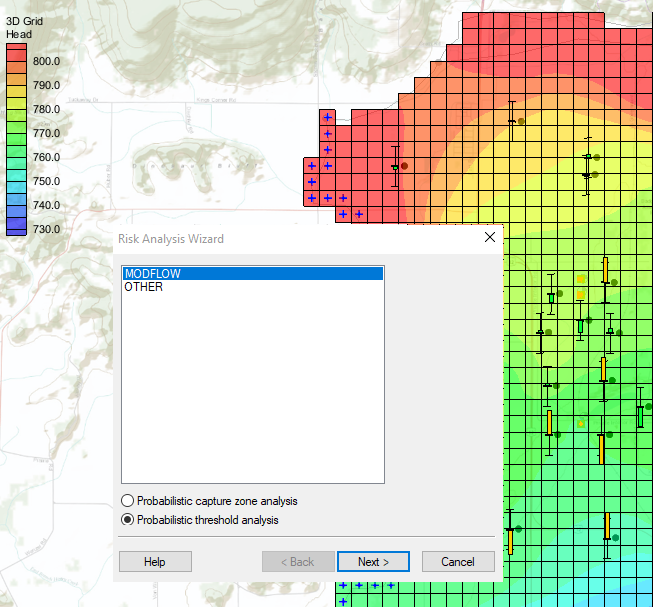
Risk Analysis for Well Groups
By aquaveo on August 3, 2022In your groundwater model, do you need a way to capture multiple wells for risk analysis? For example, your project might have multiple pumping wells and you would like to see the probabilistic composite capture zone for all wells in the wellfield. GMS provides a way to access the Risk Analysis dialog for refining stochastic modeling results.
- First open your project in GMS, making sure to select the Plan View and 3D grid module, it will be more difficult to select wells otherwise.
- Using the Select Cells tool, drag a box around the entire grid to select all cells in the grid.
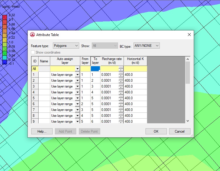
- Open the 3D Grid Cell Properties dialog and change the value for the MODPATH zone code to a number of your choice.
- Select the coverage of the well to make it active. Using the Select Points/Nodes tool, drag a box around the entire project to select all wells in the coverage.
- Select Intersecting Objects to open the Select Objects of Type dialog.
- Select 3D grid cells from the list and close the dialog. This will select all 3D grid cells that have a well in them.
- Open the 3D Grid Cell Properties dialog.
- Change the value for the MODPATH zone code to a different number than the one that was used before, close the dialog and save changes. From here, the probabilistic capture zone analysis should be able to run with the well groups setting turned on.
Please note that particles need to leave their original zone to be mapped on the risk analysis results. That is why nothing will show up when all cells were assigned to the same zone. The recommended solution is to change the zone code of just the cells with a well so that as many particles as possible can leave the assigned area.
GMS allows you to be as general or specific as you need when selecting wells for risk analysis. Try out using risk analysis for well groups using GMS today!