Aquaveo & Water Resources Engineering News

Converting External 3D Materials to 3D Grid Materials

For your 3D grid project in GMS, do you have material data from a 3D mesh or other geometry that was created in an application other than GMS? It is possible to import this data into GMS and attach it to your 3D grid using a method which involves creating solids that GMS can use to assign materials. This is done by importing the data as boreholes and creating solids from them. This post will review how you can take the material data from a 3D mesh and transfer it to a 3D grid in GMS.

To do so, do the following steps:

  1. First, you will need to import the material data as Borehole data into GMS.
  2. You will then need to create horizons for these boreholes. Go to Boreholes | Auto-Assign Horizons.
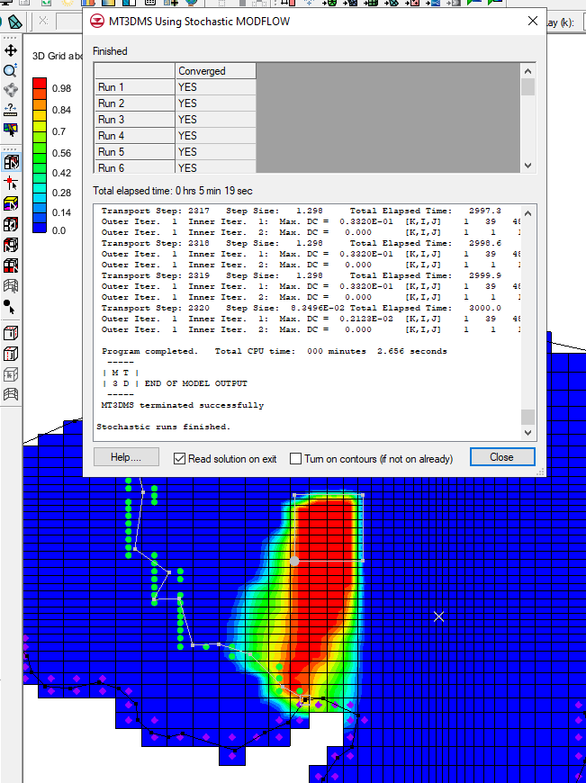
  3. In the Auto-Assign Horizons dialog, choose Start from scratch, then click Run. The Horizon Optimizer dialog will appear. This step will take a while to complete.
  4. When complete, click "Read solution on exit" and click OK to close out of the dialog.
  5. Once the Horizons are defined, click Boreholes | Auto-Create Blank Cross Sections.
  6. Once blank cross sections exist, click Boreholes | Auto-Fill Blank Cross Sections.
  7. In the Auto-Fill Blank Cross Sections dialog, select what should be matched from the auto-fill options based on the needs of the project.
  8. Cross sections created from borehole data
  9. Create a new coverage, just using the defaults should be fine in most cases.
  10. Using the Plan View and the Create Arc tool, create a closed arc surrounding all of the boreholes.
  11. Select Feature Objects | Build Polygons, to turn this closed arc into a polygon. You might also want to use the Redistribute Vertices command on the arc if needed.
  12. Turn this polygon into a TIN by using Feature Objects | Map → TIN to define the desired boundary of the solid.
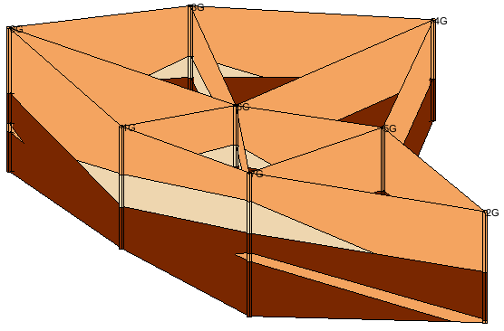
  13. Finally, create solids from the boreholes by selecting Boreholes | Horizons → Solids. This will bring up the Horizons to Solids dialog where you can choose your desired settings.
  14. The solids can then be used to classify the materials zone in place of the mesh.
  15. If the solids are needed in another project, you can highlight one or more of the solids in the Project Explorer, right-click, and Export them as a *.sol file.

Try out using this workflow to add data to your projects in GMS 10.5 today!

Blog tags: 

How to Troubleshoot Graphics Card Issues and Display Issues

Out of all the potential issues that can come up, display issues can be some of the most annoying. Display issues can come from individualized hardware configurations, display settings, operating system and software versions which makes solving these issues not as simple as a one-size-fits-all approach. This post will review general best practices for troubleshooting these kinds of issues with your graphics card or display.

Some of the most common display issues that can arise with XMS are problems with one or more of the following:

  • Transparency
  • Functional surface
  • Texture mapping
  • Film loops
  • Contours

The causes behind display issues can be divided into the following categories:

  1. Issue related to remote desktop or virtual machine
  2. Integrated graphics used instead of discrete graphics
  3. Bug in graphics drivers
  4. Limitation of integrated graphics
  5. Bug in XMS affecting all hardware configurations
  6. Bug in XMS affecting specific hardware configurations

Since hardware configurations vary and operating systems change over time, the information here is a general workflow used for troubleshooting.

  1. Remote and Virtual Machine issues: Check if XMS is being run locally or if a virtual machine/remote desktop is being used to rule out Category A.
  2. Versioning: Go to Help | About to note the XMS version, build date, and graphics library used.
  3. Try to rule out Categories E and F: Run XMS in Software Graphics Mode. If the issue is resolved in Software Graphics Mode, then the issue is related to Categories B - D.
  4. Try to rule out Category B: Go to the Device Manager for the Display Adapter. If the driver information/version for the discrete graphics matches what is shown in Help | About, then XMS is using discrete graphics. If not, go to Step 6 to ensure XMS is using discrete graphics.
  5. Device manager
  6. Update graphics drivers: Whether or not the system has discrete graphics, updating the graphics driver will solve some display problems. If the machine already has nVidia or AMD software installed, drivers can be updated through those programs. Otherwise, click the “Update Driver” button (shown in the dialog in Step 4) or Google “GraphicsCard Driver Download” using the graphics card model you have in place of GraphicsCard. Exercise caution with the links you click on. Be sure to click on official AMD, nVidia, or computer manufacturer websites. Avoid 3rd party utilities that offer to optimize your system or install adware/spyware.
  7. Set system to use discrete graphics: Change settings to ensure XMS always utilizes discrete graphics. Many systems, especially laptops, default to power saving modes where programs utilize integrated graphics even if the machine has discrete graphics. The way to change these settings varies by machine.
  8. Reporting Bugs: If Categories A - D have been ruled out, determine if the issue is machine-specific. If reproducible, report to tech support.

If you continue to experience display issues, contact Aquaveo's technical support team.

Blog tags: 

How to Rebuild a Corrupted Project in SMS

Try as we might, we can’t always make everything go according to plan, and sometimes that can include files failing on us. Occasionally, files used in SMS become corrupted and can no longer function properly.

This can happen for a few reasons. A file may have been blocked from saving correctly by the computer’s system security. The save process may have terminated early. The project files may have been copied incorrectly. The project files may have been stored incorrectly. Or some other unknown error may have occurred.

Project load error

While the corrupted project file itself cannot be restored, the component pieces of the project can be reassembled in SMS and saved out as part of a new project file. Below is a list of the file types you will need to reassemble:

  • [project name].map: These are the Map Module coverages saved to the project. The model-specific boundary conditions will likely need to be entered again.
  • [project name]_meshes.h5: These are the meshes that were in the project for models that use a mesh. Load this before loading any of the datasets saved in the [project name]_datasets folder.
  • [project name]_grds.h5: These are the grids that were in the project for models that use a grid. Load this before loading any of the datasets saved in the [project name]_datasets folder.
  • [project name].h5: This contains scatter sets that were in the project.
  • Any GIS layers, such as rasters or shapefiles, will also need to be loaded again.

For ADCIRC models, use the following files to import the ADCIRC simulations:

  • Use the fort.14 or fort.15 files to import the mesh and create the simulation.
  • Also import solution files such as fort.63, fort.64, maxele.63, and maxvel.63 files.

For CMS-Flow, use the following files to import the CMS-Flow simulations:

  • Use the [project name].cmcards file to import the UGrid and create the CMS-Flow simulation.
  • To load solutions for the CMS-Flow simulation, import the [project name].h5 files.

For SRH-2D models, use the following files to import the SRH-2D simulations:

  • Reload SRH-2D simulations (including the coverages linked to them) by loading the SRHHYDRO file, found under the [project name]\SRH-2D\[simulation name] folder.
  • To load solutions for SRH-2D simulations that were already run, import the XMDF.h5 file from the same directory as the SRHHYDRO file.

For STWAVE models, use the following files to import the SRH-2D simulations:

  • Reload STWAVE simulations (including the coverages linked to them) by loading the [simulation name].sim file, found under the simulation folder.

It is strongly recommended that a thorough review of the project should be completed before you continue working with the rebuilt project.

When your files become corrupted, please contact Aquaveo Technical Support (support@aquaveo.com) to report the issue.

If you have issues with corrupted projects in SMS, try following some of these steps to fix them in SMS 13.1 today!

Blog tags: 

Tips for Stochastic Modeling in GMS

Groundwater models often need to deal with a fair amount of uncertainty, especially when models have limited calibration data available to them. A stochastic modeling approach can be a useful option for dealing with this uncertainty by running a set of models to estimate the probability of certain outcomes, and GMS provides a few tools and methods to utilize this approach. This post will review some tips and tricks when it comes to stochastic modeling in GMS.

GMS provides three methods for stochastic modeling, using either MODFLOW 2000 or 2005. These are parameter zonation (which can be done either by a random sampling approach or a latin hypercube one), indicator simulations, and the Null Space Monte Carlo (NSMC) method.

Running a stochastic model

When parameterizing a model and identifying which model inputs need to be randomized, aim for parameters with the highest uncertainty. But make sure to not select too many parameters, as having too many selected will require substantially large numbers of model runs to complete to be able to sufficiently explore parameter combinations, and this may become unreasonable. Also make sure that when defining key values to parameter zones, you don’t use values expected to normally occur in MODFLOW input. Negative values typically can accomplish this.

When it comes to indicator simulations, T-PROGS software is generally used to generate either multiple material sets or multiple MODFLOW HUF input sets to be used for stochastic simulation. Keep in mind that only a maximum of five materials can be used with the T-PROGS algorithm. This is an intentionally imposed limitation to keep data processing and user-interface from becoming too complex. While it is a hard limit, it is generally easy to condense borehole data down to five materials or less.

Once the stochastic modeling results have been generated, you can refine the results, either with the Risk Analysis Wizard or by using the Statistical Analysis command on a stochastic folder. The latter will create datasets for the mean, min, max, and standard deviation, which can be visualized by using 3D grid display options.

More information on stochastic modeling in GMS can be found at the Aquaveo XMS Wiki or reviewing the GMS tutorials for stochastic modeling.

Try out using stochastic modeling in GMS today!

Blog tags: 

Converting a Lidar File to a DEM in WMS

Do you have a lidar file that you would like to convert into a DEM file? WMS can help you with this. Lidar files can contain a large amount of 3D points used for representing features on the Earth’s surface. DEMs can be derived from high-resolution LIDAR data, and we have developed a workflow that can do this. This post will review how to convert LIDAR files to DEM files quickly and easily in WMS.

This can be done by using the following workflow:

  1. Use any of the methods to open files to import your lidar files into your WMS project.
  2. If you have more than one lidar file imported into the GIS module, select all of the separate files and then right-click one of them and select Merge… to open the Lidar File dialog where you can name and save your merged lidar file.
  3. After you have imported your lidar file, right-click it in the Project Explorer and select Interpolate to | Raster… to open the Interpolate Lidar to Raster dialog.
  4. Review the settings and click OK when they are all set correctly.
  5. Converting Lidar to Raster
  6. In the Raster File dialog, set the name and type for the raster file and then click Save to close the dialog and save the raster file.
  7. When done generating the raster and updating the display, right-click the new raster file in the GIS module and select Convert to | DEM to open the Resample and Export Raster dialog.
  8. Review the settings and click OK when they are all set correctly.
  9. You should now have a DEM file of the same area as your lidar files. Hide everything in the GIS module to view the DEM file on its own.

It should be noted that if you have multiple lidar files, you can convert each file individually rather than merging them all together as was done in Step 2. The merge makes the final product easier and quicker to accomplish.

Try out converting lidar files to DEMs in WMS today!

Blog tags: