Happy Holidays from Aquaveo!
By aquaveo on December 25, 2019
Have you ever wondered what the difference between projection and reprojection is? Have you ever needed to convert a projection from one type to another in GMS, SMS, or WMS (collectively known as XMS)? The use of projections in WMS can be confusing, so the following should provide further clarification.
Projections can be associated with individual data objects, either in the object data file itself or in an associated *.prj file. If XMS cannot find a projection, the object will be left as "no projection," or, when new objects are created, XMS will assign the display projection to it. You can specify an object's projection by right-clicking on it and selecting Projection. Note that this projection must be the same as the original projection of the data; specifying an incorrect projection will result in data issues.
"Reprojecting on the Fly" occurs when datasets or objects from multiple projections are loaded into a project, where the x and y values would not otherwise overlap (i.e., the data would be displayed in two or more distinct locations). The different projections for these data will be "reprojected on the fly" to match the display projection such that the data objects will line up. Note that this does not change any *.prj files or the projections that are set for each object; it is an automatic function internal to XMS used for display purposes.
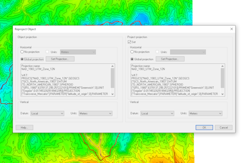
If you need to convert from one projection to another, this can be done by right-clicking on it and choosing Reproject. To use this command, the data must first have the correct projection specified. After choosing Reproject, the command will prompt the user to select a new projection, the data will be converted to the selected projection. If a *.prj file is associated with the object (such as a TIFF), reprojecting the object will change the *.prj file. Reprojection on the fly is usually sufficient for most applications. Please note that there are some limitations for reprojecting.
Once the datasets are referencing their projection correctly, XMS should reproject them on the fly to match your display projection. If you don't have a display projection set, you can do so by selecting the Display menu and choosing Projection. At that point, if you would like to reproject your scatter(s) into the same projection as the display projection, you would be able to do so.
Now that you see the differences between projection vs. reproject try them out in XMS today!
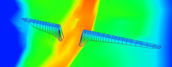
Have you ever needed to add an abutment, embankment, or other feature to your mesh and found it a struggle? We have some good news for you: SMS includes a function called Feature Stamping that is useful for this exact situation.
Feature stamping allows you to add man-made structures to an already created mesh by means of a stamping coverage.
You can find out more about this process in this wiki workflow.
There are, however, a few items to keep in mind when attempting to use the feature stamping tools. In this post, we’ll cover some of the most common, and how to troubleshoot them.
In order for feature stamping to be the most effective, it is necessary to enter them into a mesh that is already stable. Some items to look for include:
You can find much more about creating quality meshes on here our blog.
Disjointed vertices are points in the scatter that have not been connected to triangles or quadrilaterals in the mesh. Feature stamping will fail if there are any disjointed vertices in the mesh.
There are two options for fixing this:
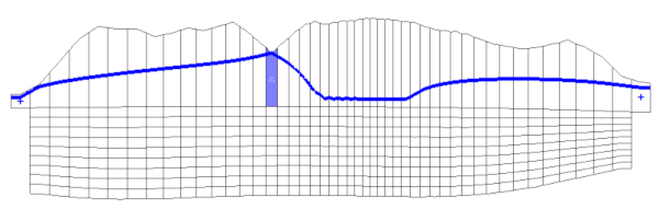
Feature stamping is usually linear, following a centerline.
If the structure is too large, or crosses over with other structures, it often has problems properly integrating with the mesh.
You can find examples here of when features are considered to be overlapping.
As long as your stamping features are reasonable in size and don’t interfere with each other, you should be able to successfully stamp your man-made features into the mesh.
Feature stamping is a very useful, but sometimes under-utilized, tool. Try out the feature stamping function in SMS today!
After completing a MODFLOW groundwater model in GMS, have you needed to see the aquifer water level? Viewing the water level can aid in visualizing the saturated thickness of an aquifer. The water level can be viewed by doing the following:
Additional information about the MODFLOW display options, including the Water Table option, can be found on our wiki.
After viewing the water table, it is possible to save the spatial 2D data for the saturated thickness (water table thickness from the aquifer base).
There isn't a shortcut way to save the 2D water table thickness. However, the desired dataset can be created by converting the head and bottom elevation datasets to 2D datasets, and using the dataset calculator to create a dataset of the difference between the two datasets. The workflow is outlined below.
Now that you know how to view and save a water table, try it out in GMS today!


