Aquaveo & Water Resources Engineering News

Using the MODFLOW HFB Package

Sometimes in a MODFLOW simulation, you need to simulate very thin barriers to flow that aren't accurately represented by assigning values to entire cells. Fortunately, MODFLOW has the Horizontal Flow Barrier (HFB) package that facilitates accurately modeling thin flow barriers. Today, we explore how the HFB package can meet your needs, and how it functions.

The HFB package can meet your need for a more realistic approach to simulating horizontal barriers in your model. Whereas many packages in MODFLOW assign values to entire cells, that might poorly reflect reality for horizontal flow barriers with negligible width. These barriers might include slurry walls, sheet pile walls, or diaphragm walls around wells. Instead of assigning values to whole cells, the HFB package uses cell boundaries to simulate horizontal barriers. Doing so can more accurately reflect the actual situation.

To use cell boundaries to simulate horizontal flow barriers, the HFB package uses a hydraulic characteristic. You calculate the hydraulic characteristic by dividing the hydraulic conductivity of the barrier by the real-life width of the barrier. This value is assigned to cell boundaries. Then, MODFLOW uses that value to modify the regular flow between cells. Thus, you get modified flow at the cell boundaries that have a defined hydraulic characteristic.
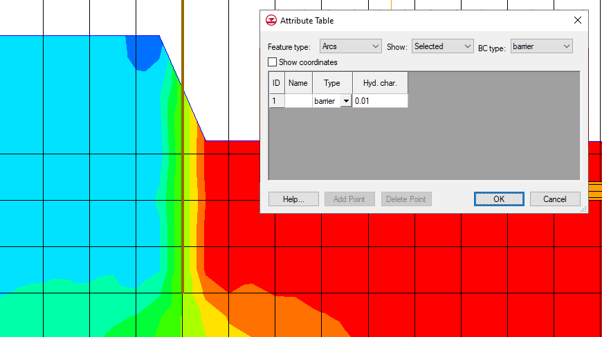
Example of the HFB Package in GMS

The following is a suggested workflow for using the HFB package:

  1. Make sure that the HFB package is turned on in the MODFLOW Packages / Processes dialog.
  2. Set up a coverage that can include a barrier by checking Barrier in the Coverage Setup. Define the layers that the barrier affects using the Default layer range in the Coverage Setup.
  3. Draw an arc representing the barrier. In the Attributes table for that arc, set its boundary condition to "barrier". Define its Hydraulic characteristic as you have calculated it.
  4. Map from that coverage to MODFLOW.

The values for the HFB package can be edited using the HFB - Horizontal Flow Barrier command in the MODFLOW menu.

While using the HFB package, keep the following in mind:

  • There are certain assumptions that this package uses to function. It's assumed the barrier has no storage capacity. It's also assumed the barrier has negligible width. Therefore, the HFB package's sole function is to reduce conductance between adjacent horizontal cells.
  • This blog post primarily applies to standard MODFLOW versions. The HFB package is also available for MODFLOW 6.

Try out the HFB package in GMS today!

Blog tags: 

Computing a Courant Number for an SRH-2D Model

Sometimes, you might want to calculate a Courant number for your SRH-2D model. In most cases, this isn't necessary because SRH-2D is an implicit model. Unlike explicit models such as HEC-RAS, SRH-2D is not Courant limited. With SRH-2D, it is more important to verify convergence and stability than Courant compliance. However, we know that calculating a Courant number dataset for SRH-2D is occasionally desired. Fortunately, SMS now has the Advective Courant Number tool to compute a Courant number dataset based on velocity.

First, let's be clear about what a Courant number does. A Courant number tells you the number of mesh elements that a given water particle passes through during a time step. If the Courant number is less than one, the given particle of water would not pass through an entire mesh element in a single time step.

In SMS, the Advective Courant Number tool computes a Courant Number dataset including every node at every time step. It uses the following equation:

Courant Number Equation

To use the Advective Courant Number tool, do the following:

  1. Make sure a transient SRH-2D solution file is already loaded.
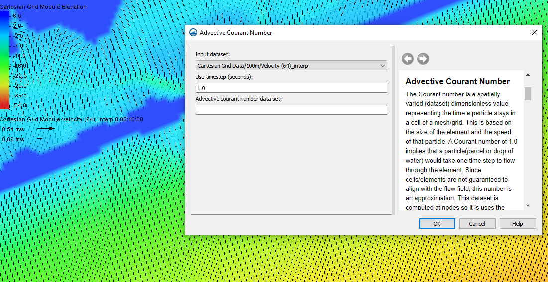
  2. Open the SMS Toolbox, and under Datasets, find the Advective Courant Number tool.
  3. Set the Velocity dataset, the time step length for the simulation, and the desired name for the output dataset.
  4. Run the tool.
Example of the Advective Courant Number tool

The Advective Courant Number tool might stall depending on the vector dataset for your SRH-2D simulation. Running the SRH-2D simulation again might solve this problem. Before running the simulation again, we recommend saving the project as a new file to preserve the old solution files. Then, in the new SMS project file, run SRH-2D again. Once the new solution is loaded into SMS, run the Advective Courant Number tool again using the new velocity dataset.

To see the results, open the Properties dialog for the Courant number dataset. There, you will find the maximum and minimum for the whole dataset and the current time step.

Calculate the Courant number dataset for your SRH-2D simulation in SMS today!

Blog tags: 

AHGW Pro for ArcGIS Pro Now in Beta!

We are excited to announce the release of Arc Hydro Groundwater Pro (AHGW Pro) for ArcGIS Pro in beta! Arc Hydro Groundwater has long helped ArcGIS users archive, display, and analyze multidimensional groundwater data. Now these same capabilities are available in ArcGIS Pro.

Arc Hydro Groundwater is a product that Aquaveo created in collaboration with ESRI. It is an add-on to ArcGIS software that enables you to work with groundwater data in ArcGIS applications. Its many capabilities include modeling boreholes and wells, creating and editing cross sections, and building 3D models.

With this new release of AHGW Pro, we wanted to highlight some of the features available.

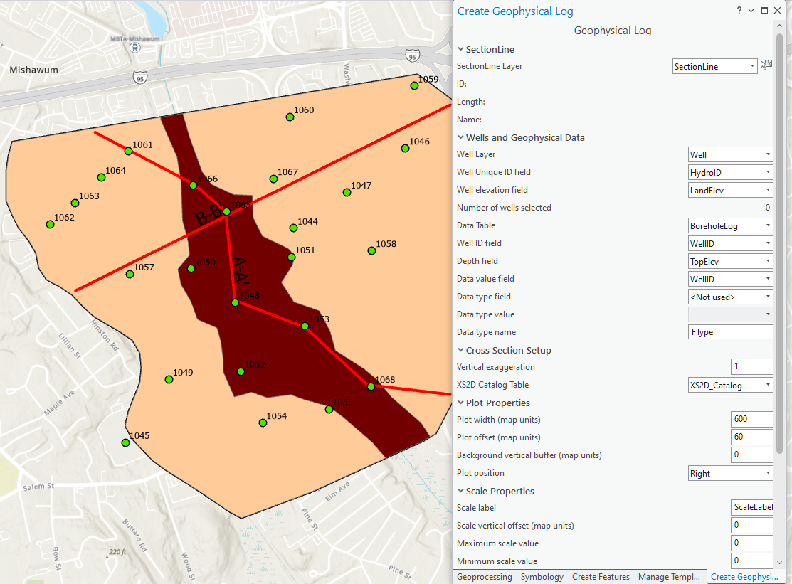
Example of AHGW Pro

For starters, you now get to combine the geodatabase technology of Arc Hydro Groundwater with the modern interface of ArcGIS Pro. AHGW Pro contains all of the tools available in AHGW with the exception of the MODFLOW analysis tools.

Another change is that ArcGIS Pro often uses panes rather than wizards and dialogs. Panes, unlike dialogs, do not have to be closed for other work to get done in ArcGIS Pro. The AHGW tools have been converted to use this pane format. This means that a tool from an AHGW Pro toolset can run while you work on something else. Furthermore, it gives you the capacity to leave the Geoprocessing pane open. Leaving a pane open preserves the last settings used in that pane. This means you can use the Geoprocessing pane to run a tool with the same settings—or slightly modified settings—more than once without having to set all the same parameters again.

Of course, you might be wary of having a lot of panes open. Fortunately, ArcGIS Pro makes it possible to stack panes, so they are neat, organized, and out of the way. You can therefore have multiple AHGW tools open while working on your project.

See what AHGW Pro and ArcGIS Pro can do together by downloading AHGW Pro for ArcGIS Pro today.

Blog tags: 

Exporting Contour Shapefiles from a 3D UGrid

Have you ever wanted to export the linear contours on a 3D UGrid as a shapefile? By exporting GMS contours as shapefiles, you can open contour shapes in other GIS applications or in other GMS projects. GMS provides functionality for exporting UGrid contours to shapefiles. This article gives some guidance for using this functionality.

In GMS, linear contours display on the top and the bottom of the 3D UGrid. This can result in contour shapefiles with undesired shapes that make contours unclear. Fortunately, GMS 10.7 can now display just one cell face (top or bottom) of single layers in a 3D UGrid. This enables exporting cleaner contour shapefiles from one face of a layer in a UGrid.

For example, GMS can display just the top of layer 1, or it can display just the bottom of layer 3. This can make for cleaner contour shapefiles because the files will have contours from only one face of the 3D UGrid. This is useful if you want the contours from a UGrid but only need the top- or bottommost contours.

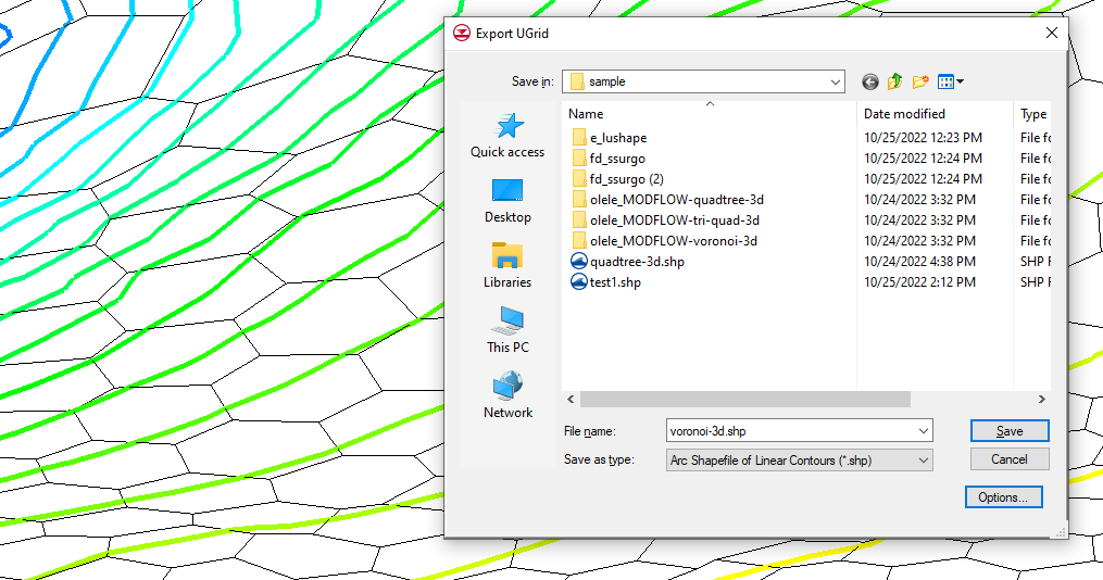
Example of exporting UGrid contours to a shapefile

Do the following to export contour lines from one face of a UGrid layer as shapefiles:

  1. Have a 3D UGrid visible in the Graphics Window. Make sure that it has a dataset that can be visualized using contours.
  2. Activate the desired dataset.
  3. Set the contours to linear in the dataset Display Options.
  4. Turn on Single layer in the UGrid Single Layer toolbar and select the desired layer. By default, the UGrid Single Layer toolbar is to the right of the XYZS Bar at the top of the GMS window.
  5. Adjust the drop-down in the UGrid Single Layer toolbar to show the cell faces desired: top, bottom, or all. GMS displays the top faces by default. This also adjusts which contours display. Now you have a certain set of contours singled out. These will be made into contour shapefiles.
  6. Right-click on the active UGrid and select Export.
  7. In the Export UGrid dialog that appears, select "Arc Shapefile of Linear Contours (*.shp)" from the Save as type drop-down and save the contour shapefile with the desired name.

If you move the shapefiles, make sure to move them with all of their accompanying files. That includes the files ending in "*.dbf", "*.prj", and "*.shx".

There may be breaks in the displayed faces of the UGrid when only showing the top or bottom face of a layer. This is because some adjacent cells are joined only by vertical cell faces; the edges of the top or bottom of the cells don't touch. Thus, when the vertical cell faces are hidden, there is only empty space. This often affects the display of the contours and the contour shapefiles.

Try exporting your UGrid contours as shapefiles in GMS 10.7 today!

Blog tags: