Aquaveo & Water Resources Engineering News

Using Arc Annotations in SMS

Have you been wanting to have more contextual information for your arcs in SMS? Some projects require being able to easily tell which direction arcs are flowing or quickly see the distance of arcs. With the release of SMS 13.1, you may have noticed an addition to the display options that can help with this. The Arc Annotations options can provide additional contextual information to arcs in your SMS projects. This post will review how they can be accessed, and how they can help you while modeling in SMS.

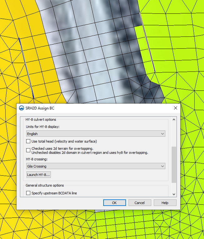
The options for arc annotations are contained within the Map tab of the Display Options dialog. The Map tab can be accessed either by selecting Map from the list within Display Options, or by right-clicking on Map Data in the Project Explorer and selecting the Display Options… command. Once in the Map tab, the Annotations option can be turned on, which will then activate an Options… button. Clicking this button will bring up the Arc Annotation Options dialog where the new arc annotation options can be selected.

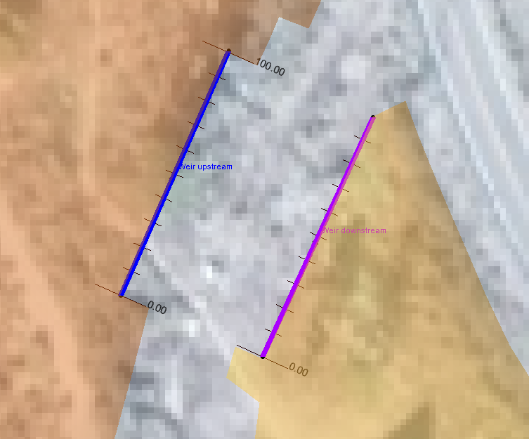
The main options that can be set here involve direction and ticks. Direction will show arrows on arcs to indicate which direction they are flowing. Ticks will show tick marks on arcs to indicate length measurements, which can help in visually seeing the real-world length of arcs. There are multiple options when it comes to how ticks will be displayed, giving you flexibility for your specific needs when it comes to modeling. It is important to note, however, that ticks will only display if the project units are set to feet or meters.

Example of the arc annotations

These features can be valuable in projects where the added visual cues and references can help with more instantaneously interpreting the graphical data. The customizability for tick display will also allow for the optimization of making this information look as presentable as possible within the model. For more details on the options available when using arc annotations, visit the XMS Wiki to learn more!

Try out using arc annotations in SMS 13.1 today!

Blog tags: 

New Features in GMS 10.6 Beta

Aquaveo is pleased to announce the release of the Groundwater Modeling System version 10.6 in beta! With this beta release, GMS contains changes and improvements to various features, much of it involving increased support for MODFLOW 6 functionality. We’d like to highlight some of the new functionality you can expect to find in GMS 10.6 beta.

Transport Support for MODFLOW 6

GMS 10.6 beta adds the ability to work with transient models for MODFLOW 6, as demonstrated by the addition of transport packages relevant to the GWT (Groundwater Transport Model) package. These will be helpful to many different aspects of groundwater transport modeling, such as dealing with advection, constant concentration, and dispersion. With the wealth of packages this alone adds to GMS 10.6 beta, it will add a lot of functionality to what GMS can do with MODFLOW 6 simulations.

Example of the new MODFLOW 6 Simulation dialog
Increased GWF Package Support MODFLOW 6

In addition to the suite of transport-related packages that GMS 10.6 adds to work with, support has also been added for more packages relevant to the GWF (Groundwater Flow Model) package. In this case, this includes the addition of the BUY (Buoyancy) and CSUB (Skeletal Storage, Compaction, and Subsidence) packages. The addition of these packages will help flesh out what GMS 10.6 beta can do with MODFLOW 6 simulations.

Support for Exchanges in MODFLOW 6

Support has also been added in GMS 10.6 for exchanges. These include the GWF-GWF and GWF-GWT exchanges. These can be used to help different models in a GMS project interact, and designate the nature of how they should interact. GWF-GWF exchanges can help two different GWF models interact together and hydraulically connect, telling each model that there is flow along a shared edge. GWF-GWT exchanges can help designate which GWF and GWT models should interact with each other.

These are just a few of the new features and changes coming out as part of the release of GMS 10.6 beta. You can find more information on what will be introduced in GMS 10.6 beta by going to the Aquaveo XMS Wiki. Try out these features and more by downloading GMS 10.6 beta today!

Blog tags: 

Making Use of WMS Contour Labels

Does your watershed project need to display contour elevations values? WMS (as well as SMS and GMS) have the ability to use contour labels to help determine elevation levels at a glance, which can be very helpful for many projects, especially when modeling drainage. This post will review the different ways that contour labels can be utilized within WMS.

Example of contour labels

There are essentially two different forms or methods when it comes to applying contour labels to contours when working in WMS: manual and automatic. In both cases, the way contour labels are displayed can be modified in the Contour Label Options dialog, which can be accessed by clicking the Label Options… button when the Contour Options dialog has been brought up. Here there are options for color, orientation, font, scientific precision, etc. There is also a button to "Erase all existing contour labels" and start over from the beginning.

The manual method consists of using the Place contour label tool to click on contours and manually assign contour labels to the positions the user chooses. This option is only available in certain modules, such as 2-D Grid and Terrain Data. Note that these may disappear when options in the Contour Label Options dialog are modified, so it may be best to determine the contour options before you manually place contour labels. Labels can also disappear when contouring options are changed, when the Graphics Window is refreshed, or can even be manually deleted when holding down Shift and clicking on a label with this tool active.

The automatic method consists of using the Automatic Labels section in the Contour Label Options dialog to automatically populate labels along the contours. When activated, this allows you to set how many of the contours should be labeled, which contour to start with, and how far apart the labels are spaced out. Unlike in the manual method, changing options for these labels should not delete them, as they should automatically repopulate based on current settings when the OK button is clicked to close the Contour Label Options dialog.

While every project will be different, when using contour labels, some recommended settings to start off with would be to use "Color Fill and Linear" as the Contour Method, and to automatically space out labels. This way more discrete contours as well as gradient values can be easily displayed and it will be easy to determine at any given location what the elevation is. Also recommended is to avoid using white text in most instances, as it is usually difficult to read, except perhaps in instances where color fill is used.

Try out experimenting with contour labels in WMS 11.1 today!

Blog tags: 

Best Practices for Extracting Features

Have you used the Extract Features tool in SMS before? The Extract Feature tool lets you generate channel and bank arcs from elevation data. There are some tricks to optimizing the use of this tool. This post will review some of the best practices that you should follow when you extract features from elevation data in SMS.

Digital Dams
Example of a digital dam

These are often artifacts from stamping channels or unprocessed LIDAR data and they can cause problems determining flow directions on the raster. The pre-processing engines (TOPAZ and TauDEM) fill these prior to computing flow directions, which can be a problem if the centerline strays from the thalweg and matching depth is computed off of the filled raster and not the original, which will also cause higher elevations along the channel above the dam. These can be fixed by either:

  • Trimming the raster above the dam by right-clicking on the raster and selecting Convert To | Trimmed Raster using a Map Module polygon.
  • Modifying elevations downstream of the dam to match correct stream thalweg elevations by right-clicking the raster and selecting Editing | Edit Raster using selected arc elevations.
Placing Points for Extracting Bank Features

When extracting bank features, place the point closest to the most important area. For example, if a section is being used for bridge analysis, place the point close to the bridge. This allows the bank lines to stay the closest to the original feature. If the Extract Bank tool misses a bank section, try moving the point to the missed section and run it again.

Extracting Centerlines for Braided Streams

When extracting centerlines for braided streams, sometimes they may not follow the actual stream location because of digital elevation model inaccuracies. When this happens, extract both centerlines and manually merge the arcs into a single arc after both centerlines have been extracted.

Use the Depth That Is Option

The following guidelines should be observed when using the "Use the depth that is" option:

  • If there is a single well-defined channel with a strong bank feature, use the "Closest to centerline" option.
  • If there are multiple floodplain bank features, use the "Closest to previous" option, otherwise, the Extract Features tool may catch a different floodplain feature.
  • If there are multiple channels or a braided stream (and you want to catch the widest extents of the channel), use the "Furthest from centerline" option.

Try out some of these best practices while extracting features in SMS 13.1 today!

Blog tags: 

Avoiding Grid Over Refinement in GMS

When building a grid for your groundwater model, it can certainly be tempting to make a really refined grid. While this temptation is understandable, there are certain pitfalls that can result from having a grid that is overly refined. This post will go over some of the reasons to avoid overrefining your grid in GMS.

There are, of course, legitimate reasons to refine portions of your grid. Portions of the grid that are key areas should be refined. This should be done only in areas around wells or other structures that are important to the model. By refining key areas, important areas of the grid will receive more attention during the model run. However, over refining your grid can cause some issues, including some of the following ones listed here.

Example of Grid Refinement

When you are refining, you are creating more grid cells in your grid. Each of these cells will be used in the model run calculation. A grid that has been over refined generally has a lot of cells that need to be used in the model calculations, many of which are unnecessary. This will cause the model run to go slower and take longer than the same model without the over refinement.

Because an over refined grid contains refined cells in unimportant areas of the project, the data from these areas can sometimes skew the results. The model run does not generally discriminate between important and unimportant parts of the grid. When it encounters a portion of the grid that has a lot of cells, it gathers all the data it can for that area. In an over refined grid, this can mean it gathers more data than the model needs, which sometimes can skew the results.

The biggest issue we most often see is when over refined grids cause the model to fail to converge. Once again, an over refined grid will have too many cells and be collecting too much nonessential data. All of this can overwhelm the model and can cause the model run to diverge. To resolve this, you will need to simplify the grid so that the model run stays focused on the key areas of the model.

Try out some of these tips while refining grids in GMS 10.5 today!

Blog tags: 

World Bank ArcHydro Groundwater Training

Recently, Aquaveo had the opportunity to participate in an ArcHydro Groundwater training organized by the World Bank. The online training happened from the 9th to the 12th of November 2021.

AHGW example

The training covered the uses and applications of the ArcHydro Groundwater (AHGW) tool used with ArcGIS. AHGW aids in displaying and analyzing multidimensional groundwater data, including representations of aquifers and wells/boreholes, 3D hydrogeologic models, temporal information, and data from simulation models.

Topics covered in the 4-day training included setting up a groundwater model and working with boreholes data. Other topics covered further included creating wells and cross sections in groundwater models, along with performing model analysis.

The training had 30 active participants in attendance from the National Water Informatics Centre (NWIC), the National Hydrology Project (NHP), the National Institute of Hydrology (NIH), the Water Resources Department (WRD) of the Indian Institute of Remote Sensing, and ESRI. For the online training, participants were located in various states in India including: Kerala, Karnataka, Uttar Pradesh, Tamil Nadu, Sikkim, West Bengal, Odisha, Telangana, Maharashtra, Gujarat, and Rajasthan.

Aquaveo would like to thank the World Bank for setting up this online training. We'd also like to thank all of the participants for their interest and efforts in using AHGW.

If you are interested in attending a training session for AHGW or any of Aquaveo's products, check out our training page for upcoming training sessions. Training sessions can be either in-person or online. Additionally, you can request a training session from Aquaveo by contacting our consulting team.

Blog tags: 

Plotting Observed Data onto a Computed Time Series Plot

Have you been wanting to make a direct graphical comparison of observed time series water-level data with computed time series water-level data? Have you been hoping to use data observed in the field to help calibrate your 2D hydraulic model in this way? While not officially supported yet, we have a workaround that could potentially help with this. This post will review how to plot both observed and computed water-level data onto the same time series plot.

There is no direct method for plotting observed data onto a computed time series graph. However, the following workflow should be able to suffice as a solution:

  1. From within SMS, bring up the File Import Wizard by using File | Open to select the file for your observed time series data.
  2. On Step 2 of the File Import Wizard, set the SMS data type drop-down to "Scatter Set", and once properly configured, click Finish to close the File Import Wizard and import the observed time series data into SMS as a scatter set.
  3. Once the data has been imported, interpolate the scatter set to your mesh by right-clicking on the scatter set and selecting the Interpolate to... command to bring up the Interpolation Options dialog.
  4. Select the scatter set data you would like and the mesh you would like to interpolate the data to, and click OK to close the dialog and interpolate.
  5. Click the Plot Wizard macro to bring up Step 1 of the Plot Wizard dialog.
  6. Select "Time Series" from the Plot Type list and click Next > to move on to Step 2 of the Plot Wizard.
  7. Select "Use selected datasets" and then click the All Off button underneath it. This will now allow you to select which specific datasets you would like to appear on the graph.
  8. Click Finish to close the Plot Wizard and bring up the Plot Window. The graph you have specified should appear.
  9. To further modify the graph, right-click on it and select Plot Data... to bring up the Data Options dialog. This will allow you to get back to the previous options and change your selection of datasets.
Example of a plot combining observed data in a computed time series plot

A future version of SMS may incorporate a more direct method for this process. But don’t let that stop you from trying out plotting observed data onto a computed time series plot in SMS 13.1 today!

Blog tags: 

Using the Axes Display in GMS

Have you tried using plotted axes to help orient the display of your models in the Graphics Window for your groundwater modeling projects in GMS? Within the Display Options in GMS, there is a set of options that will allow users to activate this and modify how it will display. This post will review how to utilize the Plot Axes functionality found in the Display Options dialog within GMS.

To locate the Axes options in GMS, open up the Display Options dialog by doing the following:

  1. Click the Display Options macro or go to the Display | Display Options... command.
  2. Select the Axes option on the left.
  3. Turn on the checkbox labeled "Enable axes" to activate the plot axes.

By default, the axes are turned off, and all the other options below it grayed out as a result. This is why axes are not usually visible on their own in the Graphics Window. Turning this option on will generate axes within the Graphics Window. The axes will naturally be sized to contain the entirety of the model within it. If the Graphics Window is currently set to Plan, Front, or Side View, rotation might be required for all of the axes to be visible.

Example of the Axes Display Options

The Axes display options allow you to control the different aspects of the axes display, such as:

  • Fly modes to set where in space the axes will be placed.
  • Tick location options to set which direction tick lines along the axes will be drawn pointing to, either inward or outward.
  • Grid line location options to set which surfaces grid lines are actually drawn on, which can help in visualizing the grid.
  • A spreadsheet containing options for editing each individual axis, as well as a row for editing all of them at once.

Try out experimenting with Axes display options in GMS 10.5 today!

Blog tags: 

Performing a Silent Install for ALS

Are you an IT administrator needing to perform a silent install of GMS, SMS, or WMS in a classroom or office? We have gone over the process to do this in the past. However, our licensing methods have changed since those instructions were first written. Because of this, we have felt it would be useful to update our users on the new method of configuration so they will be able to properly set up their silent installs. This post will review registration for the new licensing method and how to perform silent installs with it.

This silent install (or quiet install) workaround requires each user to have the rights to modify the registry. If registry access is restricted, a network administrator can do this by opening the Group Policy Management Editor and creating a startup script that automatically runs the batch file whenever the computer is restarted.

Note: Editing the Registry in Windows is a very advanced administration step. Please always create a backup of the Registry before making changes.

It can be a burden to manually update the local code in HKEY_CURRENT_USER for each user on each computer. The silent install process is simplified by creating a Windows Registry file that contains the license information and a batch file that can be executed to insert the registry information and launch WMS. The batch file automatically updates the registry for the user and then opens the WMS application. This is the safest way to edit the registry key, as well. The batch file can then be placed on each computer that needs to be updated, and the individual users can execute it as needed.

This workaround uses WMS as an example. This information also applies to GMS and SMS. You can see an example of a registry file in step 1 and the batch file in step 2, below.

  1. Create a file, "Netenble.001.reg", as follows:
    Windows Registry Editor Version 5.00M
    "ALS"="1"
    "ALSHost"="127.0.0.1"
    "ALSPort"="56789"

    ALS = 1 specifies the new registration wizard, with new "Local" codes beginning with L, F, or E, instead of 0 for the old network lock. ALSHost = 127.0.0.1 because the code is being located on the local machine. And ALSPort = 56789 should be the default - you can alternatively specify your own port if you would like. You could also specify an ALSCode (license code) as well if you don’t want registration to be required when first launching WMS.
    Note: This information was created using Windows 10. Because different Windows versions can have different REG file formats, we recommend you install WMS on one machine, register it to the correct local code, then export the registry key. Open the registry file in the text editor and remove every line except those similar to those shown in the image above, and save the file as "Netenble.001.reg".
  2. Create a file, "wms11.bat", that will update the registry and start WMS:
    reg import Netenble.001.reg
    wms.exe
  3. Place these two files in the WMS folder in the image that will be distributed to the affected computers. For example, for the 64-bit version of WMS 11.1, the default location for the folder is “C:\Program Files\WMS 11.1 64-bit\”.
  4. Create a desktop shortcut to the batch file for the convenience of the user. If doing this via a startup script in the Group Policy Management Editor, this step can be skipped.

This silent install workaround can save you significant time as a network administrator. If you experience issues while performing a silent install, feel free to contact Aquaveo for assistance.

Associating HY-8 Files with SMS

Have you wondered about how HY-8 interacts with SRH-2D in SMS? This post will review what HY-8 and SRH-2D are doing as they interact with each other.

SRH-2D has an option to use the HY-8 software to define culverts. Using the HY-8 software allows for greater definition for the culvert as opposed to defining the culvert directly in SMS. The Launch HY-8 button in the SRH-2D Assign BC dialog creates the HY-8 file and associates the file with the culvert arcs and SMS project. It is important to keep this file with the SMS project, otherwise the HY-8 file may become unassociated with the culvert.

Multiple culverts can be in the same HY-8 file, so be certain the correct culvert has been associated to the culvert arcs in SMS.

SRH-2D culvert using HY-8

When assigning properties to arcs that have been set to a BC Type of Culvert HY-8, there is a checkbox option to turn on 2D terrain for overtopping. When this is unchecked, SRH-2D will create a *_HYn.dat for the crossing. When this is checked, SRH-2D will instead create an *_INTERNALn.dat file for the crossing. In this case, SRH-2D will use the HY-8 table, but won’t see the structure as a HY-8 culvert, but as essentially a link structure.

Typically, the overtopping option is used when overtopping flow is expected to travel in a different direction from the rest of the flow. If the flow over the culvert and the flow in the culvert are both flowing in the same direction, it is not recommended to use 2D Overtopping. This is because the link structure in SRH-2D can get flow from both upstream and downstream of the boundary arc and the flow coming out of the downstream arc can go in any direction.

When SRH-2D runs, it will generate output files that are sent to an Output_MISC folder in the file directory of your current SMS project. Here, HY-8 culvert report files and/or pressure flow overtopping report files should be found, following the respective naming schemes of “*_HYn.dat” and “*_INTERNALn.dat”. The “*” is a placeholder for the specific case name specified in the model control, and the “n” will be replaced with a number in a series, for as many relevant zones or arc pairs exist in the series. We unfortunately don’t have any control over the naming convention SRH-2D uses.

More information about the different types of SRH-2D output files that may be put out after an SRH-2D run can be found here at the Aquaveo XMS Wiki.

Try out using HY-8 with SRH-2D in SMS 13.1 today!

Blog tags: 

Pages