Aquaveo & Water Resources Engineering News

Viewing a 3D Bridge in a Plot

Have you had difficulty determining where in your plots your 3D bridges are located? At times it can be challenging to determine where objects lie along a generated line plot. This is why SMS has the functionality to be able to tell the plot to display the location of a 3D Bridge. This post will review how to view the location of a 3D bridge in a plot.

3D bridge plot example

The Plot Data coverage provides the ability to locate structures on a profile plot, which could be used to map the location of a 3D Bridge. However, SMS also allows using the Bridge coverage to help see where the 3D bridge is located on the profile plot. It is important to note that a 3D bridge defined within a 3D Bridge coverage will have to be used, as a UGrid will not suffice.

Once you have all your 3D bridges created and defined, you will need to make a profile plot. This is done by using an observation arc within an Observation coverage that intersects the 3D bridge so that it will eventually be visible in the plot. Select that observation arc, and then right-clicking the arc, you must select the Show Observation Plot command to open a Plot window. This plot will automatically update based on which of the datasets and time steps are selected. This plot shows the data values along the observation arc, but by default does not show where a 3D bridge or other structures intersect with the observation arc.

After the profile plot has been generated, right-click within the Plot window and select the Plot Data command to bring up the Data Options dialog. Notice the options in the Components section related to the 3D bridge coverage. Turn on the check boxes for the 3D bridge coverage in any of the relevant rows.

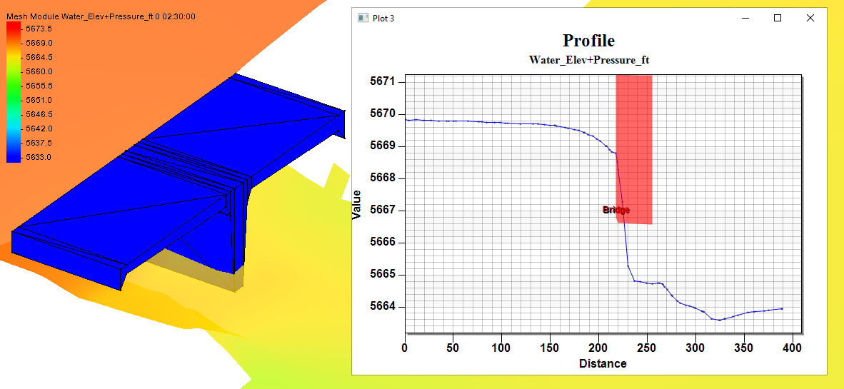
When everything has been set up correctly, the plot will have properly updated itself and you will be able to see a representation of the selected 3D bridges within the Plot window at this point. Now you will be able to properly keep track of where your 3D bridges come into contact with your profile plots.

Try out viewing 3D bridges in a plot in SMS 13.1 today!

Mapping Multiple Coverages in GMS

Do you have a conceptual model project in GMS where you have multiple map coverages with values for the same MODFLOW package? Are you wondering how GMS maps values from multiple coverages over to the MODFLOW packages?

It's not unusual for some projects to require the same attributes to be in separate coverages rather than having all the attributes in a single coverage. For example you might want to use recharge attributes from different sources and have placed the values on different coverages. But how exactly does GMS handle this? This post should hopefully give you a better sense of what GMS is doing behind the scenes.

Normally, the values for a particular MODFLOW package, such as recharge, are placed on one coverage that uses multiple polygons. In this case, a single value can be calculated, taken only from the predominant polygon, as it is expected that the polygons will all be within the same coverage. Also in this case, the methodology is designed to accommodate polygons being used to calibrate recharge zones in PEST, as opposed to calibrating with pilot points. If using gradient recharges, it is recommended to use scatter points to interpolate recharge values to MODFLOW layers.

You may have a case where you have the values for a package, such as recharge, on polygons on different map coverages. This could be because you imported the values from different sources. In cases where the polygons on different map coverage overlap, the attribute types with different values will have those values summed up when they are applied all at once if you map all of the coverages at the same time. If you don’t want them summed up, make sure that rather than applying them all at once, the value you want is the last value mapped over. This is because when multiple coverages are applied at once, GMS sum the values cumulatively, but when done individually, GMS overwrites the value with the most recently mapped coverage.

Mapping multiple coverages

It is important to note that hydraulic conductivity is not cumulative, though the sources may be. Hydraulic conductivity is overwritten every time, so the values MODFLOW receives are the values of the last polygon that intersected an individual cell.

Items in the Project Explorer are mapped in descending order, so changing the order of the coverages can change the end results.

You can also find more information on how objects are mapped to MODFLOW at the Aquaveo XMS Wiki.

Try mapping multiple coverages in GMS 10.5 today!

Blog tags: 

Viewing Multiple GSSHA Scenarios in a Hydrograph

Have you needed to compare multiple GSSHA scenarios using a single hydrograph? New functionality has been added to WMS that now allows for hydrographs that can display results from multiple GSSHA scenarios. This post will review how multiple GSSHA scenarios can be added to hydrographs, a feature newly introduced in WMS 11.1.

Hydrograph showing multiple GSSHA scenarios

Hydrographs that show multiple GSSHA scenarios plot them all out within the same hydrograph. A legend below the graph will indicate which GSSHA scenario run is which in the hydrograph, as each run should be in a different color and potentially a different line style. The dimensions of the hydrograph will be such that all of the different runs will all be able to be displayed.

To be able to work with hydrographs that show multiple GSSHA scenarios, multiple GSSHA scenarios will need to be loaded into WMS to be compared with each other. This can be done by loading multiple GSSHA projects that use the same area into WMS. These can be saved together as a single GSSHA Group Project (GGP) file if needed.

When these GSSHA scenarios will be run, rather than using the typical Run GSSHA command, instead go to the GSSHA | Run GSSHA Group Command. This will open up the Save and Run GSSHA Group dialog. Here, the projects that will run can be selected, as well as the group filename. When the projects have been selected, clicking OK will close out the dialog and bring up the Model Wrapper dialog. This will be brought up for every scenario that will be run, along with the necessary loading of the data into WMS. This will likely take some time, depending on the nature of the GSSHA scenarios, the amount of data to be loaded in, and the amount of different scenarios that will all need to be run.

Once the entire group of GSSHA scenarios has been run, selecting the hydrograph for viewing should display plots of all of the relevant hydrograph scenarios that have been run. Feel free to examine the data, and potentially experiment with different combinations of geographically related runs.

Try out multiple scenario hydrographs in WMS 11.1 today!

Blog tags: 

Using SRH-2D Monitor Plots and Structure Plots

With the release of SMS 13.1, we have added the ability to generate monitor plots and structure plots from the solution of a successful SRH-2D model run. This post will offer a brief rundown of these new features and a brief explanation of how to use them.

SMS now has the ability to generate solution plots at monitoring locations or structure locations, using solution datasets generated during the model run. If you make any edits to the coverage after running SRH-2D, make sure to rerun SRH-2D with the updated coverage to keep the plots consistent with the SRH-2D outputs.

For both plots, they will be displayed in an SRH-2D Solution Plots dialog, and they will have similar options in both cases. These options include:

  • Simulations: contains a list of all available simulations where the monitor or boundary conditions coverages were included during the simulation run. Select which solution set to use for the plot.
  • Plots: contains a list of all available solution datasets from the model run. Datasets you select will appear in the plot.
  • Specify time range: specify the time range for the plot to display. The possible range will be from 0 to the length of the entire simulation.

To use the monitor plots:

  1. Make sure you are in the monitor coverage and select a monitoring point or line.
  2. Right-click to select the Monitor Points Plot or Monitor Lines plot command.

This will open the SRH-2D Solution Plots dialog. Note, you need to make sure the monitor coverage was included in the simulation run, and that only one point or line is selected.

To use the structure plots:

  1. Make sure you are in the boundary conditions coverage and select a structure arc.
  2. Right-click to select the Structure Output Plots command.

This will open the SRH-2D Solution Plots dialog. Note that you need to make sure the boundary conditions coverage was included in the simulation run, and that only one structure arc is selected, even for structures that require two arcs.

Structure plot example

Try using monitor plots and structure plots in SMS 13.1 today!

Blog tags: