Comparing SRH-2D and HEC-RAS Solutions
By aquaveo on May 25, 2022Have you ever wanted to compare model results between SRH-2D and HEC-RAS models? The SMS 13.2 interface allows you to view both SRH-2D and 2D HEC-RAS results for the same model at the same time.
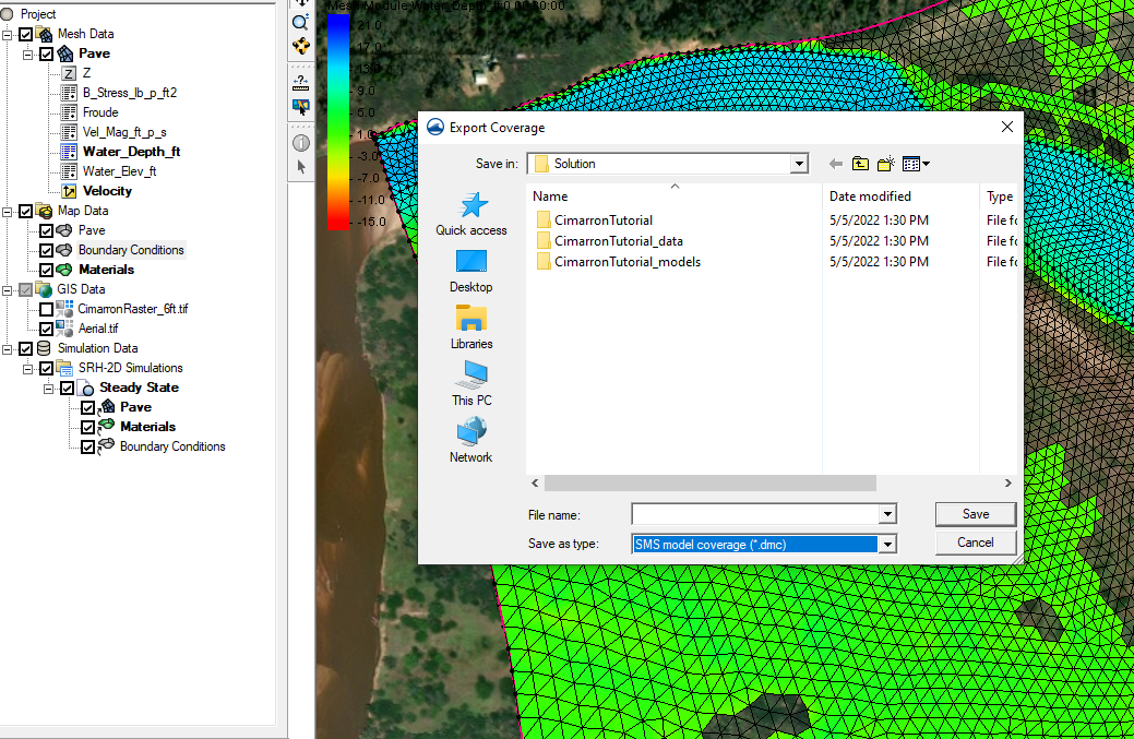
Say, for instance, that you have created an SRH-2D simulation in SMS and you want to compare results using HEC-RAS. First, if you do not have the project in both SRH-2D and HEC-RAS, you will need to create an HEC-RAS simulation in SMS and use it to export the SRH-2D mesh into a file format that HEC-RAS can use. Then you can import the mesh into HEC-RAS and set up the boundary conditions and other attributes of the simulation.
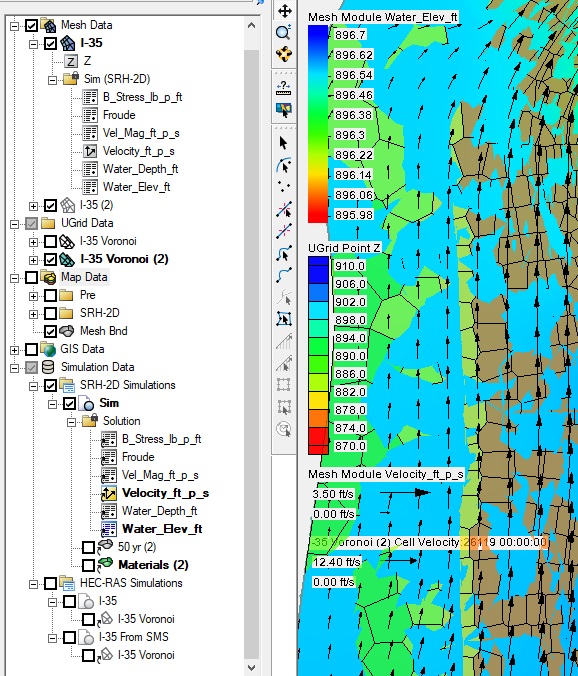
Once you have a completed simulation for both SRH-2D and HEC-RAS, you can import the results of the HEC-RAS simulation into the SMS project containing the SRH-2D solution. To do this, simply open the "*.p**.hdf" file generated by HEC-RAS in SMS. This will import the HEC-RAS solution into your SMS project. The HEC-RAS simulation solution will appear on a 2D UGrid.
There are many different comparison options available, a few are listed below:
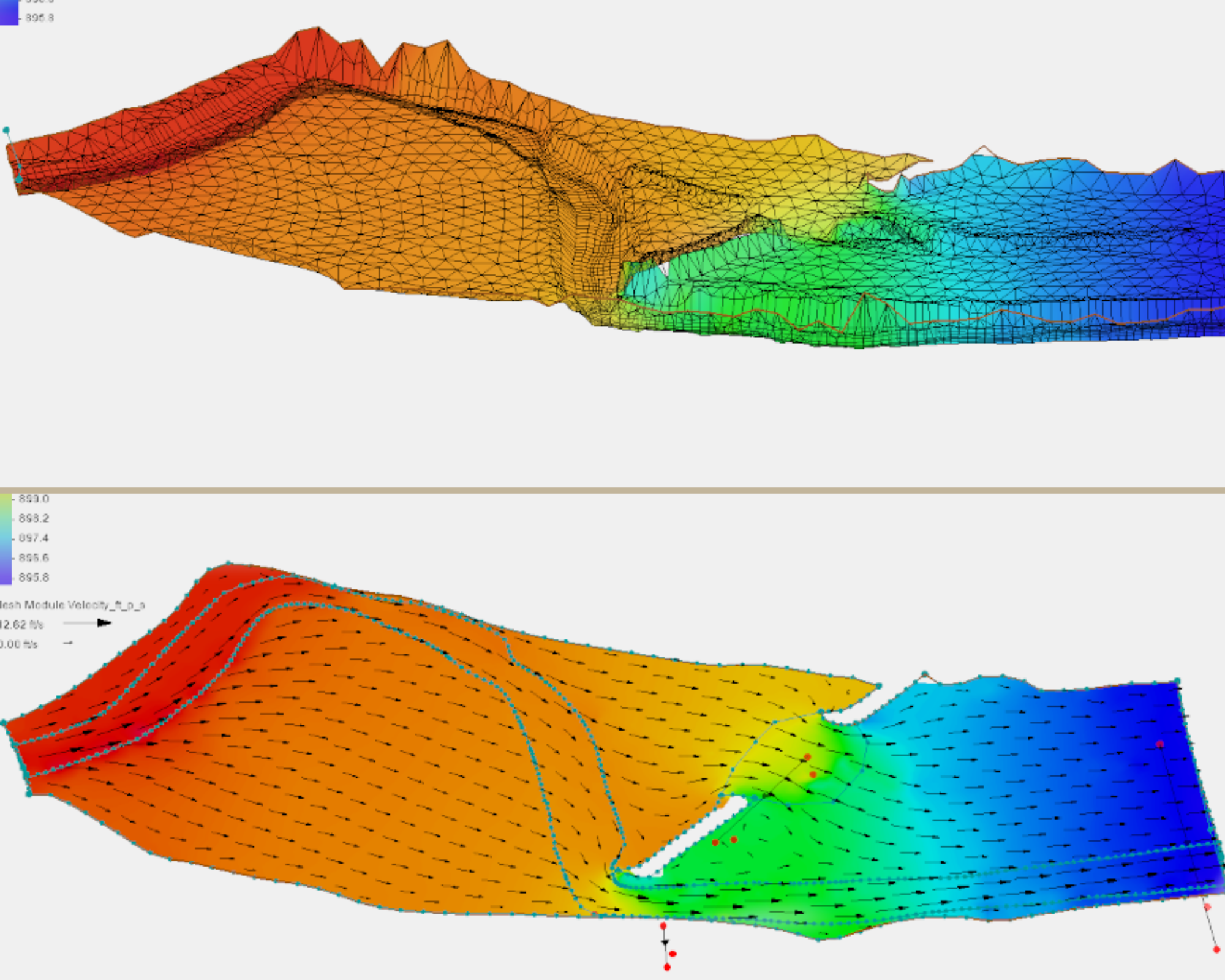
- The first comparison is often a quick visual check. Switching between the two models in the Project Explorer will let you make quick visual comparisons. You may need to adjust your contour display options to make this easier.
- Using the Data Calculator, you can make a comparison dataset. Since the HEC-RAS solution will be on a UGrid and the SHR-2D solution will be attached to a 2D mesh, you may need to convert data to be in the same module in order to do this.
- Observation Plots are another way to compare the models. You can plot the solutions from both models using the same observation coverage.
Try out comparing SHR-2D and HEC-RAS models in SMS 13.2 today!