Aquaveo & Water Resources Engineering News

4 New Features in the GMS 10.4 Beta

We’re happy to announce the beta version of GMS 10.4 is now available. Our developers have been working hard to improve GMS to make the user experience more enjoyable.

To help you learn about some of the new features, we’ve compiled this list of four new features in GMS 10.4 Beta.

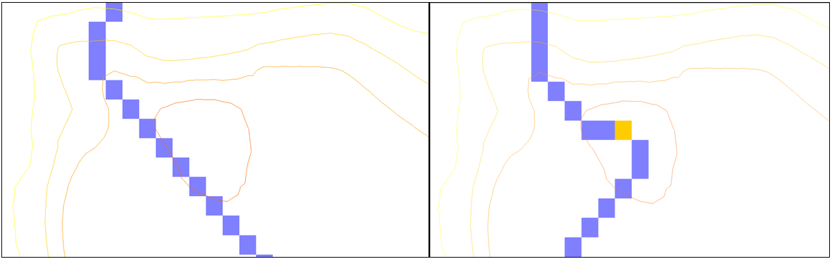
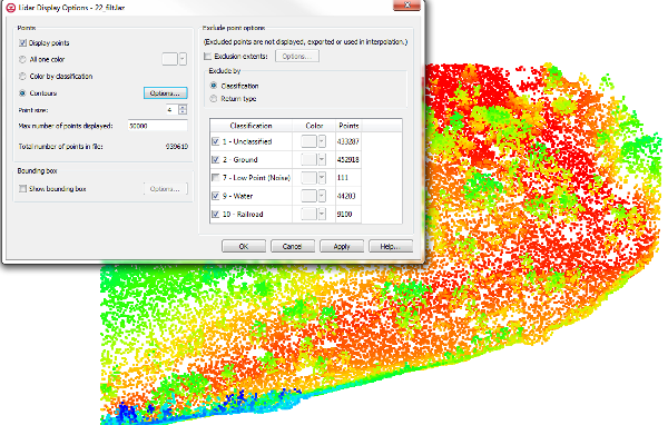
  1. New tools to support the use of lidar data. You might have used lidar files in the past and noticed that the interface was a little confusing and sometimes slow. After examining how the process could be improved, we made improvements to the import process and changed how GMS interacts with lidar data. We hope you find our new lidar functionality is both faster and makes working with lidar data easier.
  2. MODFLOW-USG Transport can now be used with GMS. This version of MODFLOW allows including transport modeling into your projects. With it comes the Block Centered Transport (BCT) process, Dual Porosity Transport (DPT) package, and Prescribed Concentration Boundary (PCB) package. Other options are also included in the MODFLOW-USG Transport model to give a wide range of access.
  3. Head observations for Connected Linear Network (CLN) wells can now be created to measure the computed head in a CLN node or cell. The process is similar to creating head observations in the groundwater domain with some differences. Overall, CLN observations are simple to create and provide a great addition to the CLN process.
  4. You can now export your MODFLOW project for use with MODFLOW 6. This is done similar to saving native text files.

These are only some of the many new and updated features in GMS 10.4 Beta. You can find a bigger list of them here. Along with these new features, we are also excited to offer new tutorials instructing users on how to best utilize the new features. There are specifically tutorials on the new features listed above. Try out the beta by downloading it today!

Blog tags: 

How and When to Use Depression Points in WMS

Have you ever wondered what depression points are used for? Should you be including them in your watershed delineation? Depression points can greatly help to improve the accuracy of your model when used correctly.

A depression point is significantly lower than its surrounding elevation, causing a change in flow accumulation and direction. An example of a depression area would be a watershed that contains a mine. TOPAZ is a public domain program that is used in computing flow directions and accumulations for use in basin delineation with DEMs. TOPAZ assumes that all depression points it encounters in its calculations are due to a lack of resolution, and therefore “fills” the depression point in increments until a flow path can be established straight across the low point. In order to view how a natural depression point would affect flow direction and accumulation, it is necessary to define the specified areas as depression points. This causes TOPAZ to read the cell as a NODATA cell, making TOPAZ think it is a DEM boundary instead of raising the elevation in the depression. Comparing a before and after of marking a depression point shows how the flow path is affected by depression points as displayed below.

It is appropriate to use a depression point where a natural depression occurs in the horizon. Typically you would only define depression points for larger areas where the flow path will be significantly affected by the area. It is not always necessary to define a depression point however. You want to use it when you receive straight lines for delineation boundaries for instance. This would most likely be caused by undefined depression points.

Some errors can occur however when defining depression points incorrectly.

  • Sometimes users will mark the bottom elevation that is actually up higher to the side of the depression point and is not exactly the center deepest point. This issue can be avoided by using the Set contour min/max tool in the Terrain Module to correctly identify the absolute bottom elevation. This DEM point is the one which should be marked as a depression point.
  • Another incorrect use of depression points would be to use them to outline where a stream bed is. A stream bed can be identified by using stream arcs in WMS.

Now that we’ve established when and when not to use depression points, you might be wondering how to create depression points in WMS. To create depression points in WMS:

  1. Turn on the Terrain Data Module.
  2. Use the Select DEM points tool to select the cell containing the lowest DEM elevation. If working with an area that has a large natural depression, simply hold down the Shift key to select all of the cells with low elevation at once.
  3. Select DEM | Point Attributes to bring up the DEM Point Attributes dialog.
  4. Turn on Depression point to mark the cell as a depression point.

Now that the depression points are set, you can run TOPAZ to view the new flow paths. TOPAZ will recognize the new depression, and the detention basin calculator can be used to create a stage-storage curve.

Try adding depression points in your WMS model today!

Blog tags: 

Creating SRH-2D Pressure Zones with Overtopping

Do you have a location in your SRH-2D project for a box culvert or pressure zone with overtopping?

It is a common feature added to many SRH-2D models. Depending on how the pressure zone is created in SMS, this can be a tricky process for SRH-2D to handle. Here are some steps and tips for creating this feature successfully in SMS.

1 Use Quadrilateral Elements

Create quadrilateral elements between the boundaries of the pressure zone. Using quadrilateral elements tends to increase the stability and reliability of the SRH-2D model run. Quadrilateral elements can be created in one of two ways.

The first is to create the quadrilateral elements when creating the 2D mesh. Create a polygon for the area between and around the pressure zone. Assign this polygon with the Patch mesh type in the 2D Mesh Polygon Properties dialog.

The second method is to create the quadrilateral elements directly in the mesh using the Split/Merge tool and the Switch Element tool. This can be time-consuming, so it is only recommended for small adjustments.

2 Create Voids

Create voids in the mesh on either side of the pressure zone. There are two options for creating these voids, but one option seems to work better.

The first option, and the more stable one, is to create the voids on either side of the pressure zone when generating the mesh. Create the voids as polygons and assign them the None mesh type.

The second option is to generate the mesh then use the Select Elements tool to select and delete the elements where the voids should be. Using this method requires renumbering the mesh nodes. There is a risk that you will not be able to delete all of the nodes related to the elements which can make your mesh unusable to SRH-2D.

3 Assign Boundary Conditions

Two arcs are needed to define the pressure zone. Each arc should be created on an SRH-2D boundary condition coverage. When creating the arcs, make certain all 2D mesh elements between the arcs are quadrilateral elements. Also, it is advisable to have at least one row of quadrilateral elements just past the downstream arc.

Once the arcs have been drawn, select both arcs and open the SRH-2D Linear BC dialog. Set both arcs to the Pressure type and turn on the Overtopping option.

Both the boundary condition coverage and the 2D mesh can be added to your SRH-2D simulation to have a pressure zone with overtopping included in the results.

Try out adding a pressure zone in the community edition of SMS today!

Blog tags: 

Creating a Raster from MODFLOW Contours

You’ve just finished successfully running a MODFLOW simulation in GMS and you are viewing the results in lovely contours on your screen. Now you would like to save those results as a raster file you can import into another application.

In order to save the MODFLOW contours as a raster, the MODFLOW results will first need to be converted to a scatter point set, then the scatter point set can be made into a raster.

Converting MODFLOW Layers to Scatter Points

To convert MODFLOW data to scatter point data, do the following:

  1. Select the MODFLOW simulation.
  2. Use the Grid | MODFLOW Layers → Scatter Points menu command.
  3. In the MODFLOW Layers → Scatter Points dialog, you can select the Computed Heads option.
  4. With the Computed Heads option active, you can select the MODFLOW solution datasets and time steps to convert into a scatter point.

Once done, you will have a scatter point set in the Project Explorer containing dataset generated from your MODFLOW results.

Converting Scatter Points to Rasters

Now that you have your MODFLOW solution datasets as scatter point data, you can do the following to convert them into a raster file.

  1. In the Project Explorer under the scatter point set, select the dataset created from the MODFLOW solutions.
  2. Right-click on the scatter point set in the Project Explorer, and select Convert To | New Raster.
  3. In the Scatter → Raster dialog, set the interpolation option you wish to use and specify the extents of the raster.
  4. Finally, save your raster file with a name and raster file type.

The raster file will be loaded into GMS, so you can compare it to the contours in your MODFLOW solution datasets. The raster file contains elevation data that was in the MODLOW solution.

Now that you know how to generate a raster file from MODFLOW contours, try it in out in GMS today!

Blog tags: