Aquaveo & Water Resources Engineering News

Understanding SRH-2D's Monitor Coverage

Being able to determine hydraulic parameters at specific locations in the model domain is a handy, and sometimes even necessary, tool for any SRH-2D model. That is why there is a specific coverage in the Surface-water Modeling System (SMS) where you can create monitor objects that will collect the information you need during the simulation run. This blog post will cover some information that you may find useful when trying to make the most out of your monitor coverage.

SRH-2D outputs monitor data at a fixed interval of every 100 time steps. This is important to keep in mind if you’re looking to collect a certain amount of data from your monitor points or lines. You may need to adjust the size of the time steps depending on what kind of output you need.

SRH-2D monitor points output file
Monitor Points

When creating monitor points on the SRH-2D monitor coverage, it is recommended that you create at least three monitor points: one near each end of the model domain, and one in the middle. During the simulation run, SRH-2D collects data at the points about a number of things, including but not limited to: the position in the X and Y direction, bed elevation, water elevation, and water depth.

Monitor Lines

Monitor lines can help you verify the continuity and model stability of your SRH-2D simulation. SRH-2D uses monitor lines to calculate the total flow and average water surface elevation along the arc. Monitor lines work best when they cross a river rather than running parallel. Lines with too many curves can cause difficulties in snapping to the mesh properly. Monitor lines can be placed anywhere along a river, but we recommend that one be created near the inflow and outflow boundaries. Remember to use monitor lines judiciously. Too many monitor lines can bog down your simulation, or even keep it from converging properly.

Monitor Output Files

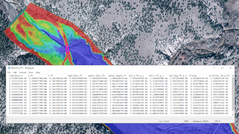
Monitor output files are automatically exported to the location of the project files using this directory format: \[Project_Name]_models\SRH-2D\[Simulation_Name]\Output_Misc. The Output_Misc folder contains a DAT file for each of the monitor features using the *[Simulation_Name]_LNn.dat naming convention for lines, and *[Simulation_Name]_PTn.dat for points. These files contain all the data for each individual point or line, and can be opened in your prefered text editor application.

SRH-2D Solution Plots

We covered how SRH-2D solution and monitor plots work in a blog post a while back. If you’re interested in learning more about solution and monitor plots and how to use them, follow this link to our website.

Head over to SMS and try out the monitor coverage with your SRH-2D model today!

Blog tags: 

Introducing HydroGeoSphere with GMS

The Ground-water Modeling System (GMS) 10.8 beta includes a model interface that is brand new to the software. HydroGeoSphere (HGS) is a unique three-dimensional control-volume finite element simulator developed by Aquanty that is meant to be able to handle all parts of the terrestrial water cycle. It uses a globally-implicit approach to simultaneously solve the 2D diffusive-wave equation for overland/surface water flow and the 3D form of Richards’ equation for variably saturated groundwater flow. This is different from the many other models that simulate only a portion of the hydrologic cycle. HGS includes components for precipitation, evaporation, overland flow, infiltration, recharge, and more. HGS can simulate both surface and subsurface water flow simultaneously for each time step.

In GMS, the base components for an HGS model include: an unstructured (UGrid), HGS coverages, and an HGS simulation. GMS allows multiple HGS simulations to exist in a single GMS project. A 3D UGrid of the project area is required before building an HGS simulation. There can also be multiple UGrids in one project, although only one UGrid can be assigned to each simulation.

The coverages specific to HGS are boundary conditions, observations, and hydrographs. GMS uses feature objects to define the boundary conditions on an HGS boundary conditions coverage. This includes points, arcs, and polygons. The observations coverage allows you to set observation points that will collect time series information during the simulation run. The hydrograph coverage records hydrograph data during the simulation run.

HGS defines materials with domains and zones. The domain contains information about the type of material. The domain is then assigned a zone number, which is then assigned to a polygon. Multiple domains can be assigned to the same zone.

HGS with GMS

There’s a lot more to HydroGeoSphere than we can cover in one blog post. If you’d like to learn more about HGS, Aquanty has numerous resources on their website. You can look at the HGS Theory Manual or the HGS Reference Manual. They regularly post webinars on their blog and on their LinkedIn. You can also find videos about how to use HydroGeoSphere as well as presentations that have been made by Aquanty’s staff on their YouTube page. We also have our own HGS tutorials that can walk you through the steps of building an HGS model.

We hope you’re excited about the addition of HydroGeoSphere into GMS 10.8, because we certainly are! Download GMS 10.8 to try out HGS today!

Blog tags: 

Defining Elevation and Storage Capacity of Detention Basins

Did you know that the Watershed Modeling System (WMS) has a calculator that can define the relationship between the elevation and storage capacity of a detention basin? This is a useful tool for any WMS project with detention basins. The detention basins calculator is a simple tool that can quickly get the storage calculations you need for your model.

WMS uses the Hydraulic Toolbox to perform these calculations for the detention basin calculator. To open the detention basin calculator, first you need to make the Hydrologic Modeling Module active and select an outlet. Detention basins… is one of the options under the Calculator menu. After selecting Detention basins… a dialog named Detention Basin Hydrograph Routing will appear. Clicking the Define… button opens the Storage Capacity Input dialog, which is where you can enter the data that is needed for the calculations.

Basin Calculator in WMS

There are four data input options you can use to calculate storage capacity in the Storage Capacity Input dialog. Only one of the four input options is needed in order to perform the calculations. Which one you use will depend on what data is readily available for your model.

It is important to note that regardless of what measurement the general display projection is set to, the detention basin calculator will measure the elevation in feet and the storage volume in acres per foot.

After you exit the Storage Capacity Input dialog, a plot will be automatically generated in the Detention Basin hydrograph Routing dialog. This plot displays the relationship between the elevation and the amount of storage, as well as discharge if there is any. This plot functions the same way as any other plot window in WMS. You can learn more about plot windows by following this link to our wiki.

Head over to WMS to check out the detention basin calculator and see how you can use it to calculate the storage versus elevation for your detention basins today!

Blog tags: 

Handling Depth vs. Elevation

When creating a surface-water model, your model will make use of bathymetry data as either elevation or depth. Knowing how the Surface-water Modeling System (SMS) represents depth versus elevation is vital when it comes to creating, running, and understanding a model. SMS uses several different numerical models, and some models require that depth be negative and elevations be positive, while other models require the opposite.

It can become confusing when trying to remember what is needed for each model, which is why the decision was made to standardize how SMS treats elevation and depth across all models. SMS treats all depth values as negative and all elevation values as positive. That way you don’t have to remember how data needs to be entered for each model. If depth data is entered with positive values, SMS will read the data as part of the land elevations, which will produce incorrect calculations.

Depth/elevation shown on a grid

Some of the most used models where you may see that the elevation values have been changed to fit SMS’s conventions after importing are CMS-FLOW, CMS Wave, and CGWAVE. If you’re not sure whether or not the imported elevation data has been changed and would like to check, then this is a great time to make use of the Mesh module’s find function. Under both the Nodes menu and the Elements menu you’ll see a Find… option listed. You can use this to quickly locate a specific node or element inside of SMS to compare the elevation data with the model’s files outside of SMS.

If SMS has changed the values of the elevation data to account for the required negative depth value, there is no need to be concerned about how this will affect the end result for your model. SMS automatically adjusts the data to match the convention of the model when the project information is exported to the model executable.

Take this information and head over to SMS, more confident that your project’s elevation data will be handled correctly.

Blog tags: 

Troubleshooting MODFLOW in GMS

When constructing a MODFLOW model in GMS, there is always the possibility that you will get an error when trying to run your model. While there are a number of things that could be keeping your model from running without an error, here are some tips to help you figure out what may be going wrong.

Example of the MODFLOW Model Checker

Before running MODFLOW, make use of the Model Checker. The Model Checker will analyze all the current input data for any obvious errors or potential problems, which could save you from having to hunt down individual input errors. The Model Checker gives you a few options for sorting and displaying errors. The Model Checker is a useful tool for a basic check of the inputs, however the Model Checker coming up clean doesn’t necessarily guarantee that the solution is correct.

Example of the MODFLOW Model Checker 
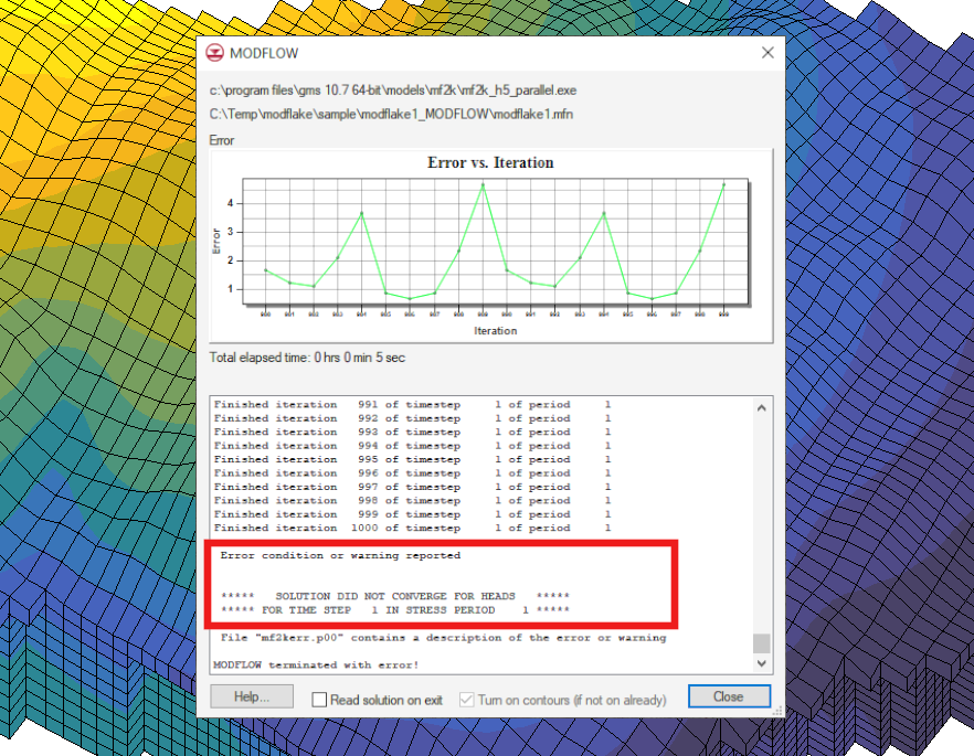
The next thing to look at in your MODFLOW model when you’re trying to figure out what the issue may be is the command line output from the MODFLOW model wrapper dialog. When the model does not converge, an error message should appear in the command line output. This message will help you know where to start resolving the issue.

Another place to look when you’ve encountered an error is the MODFLOW output file (*.out) in the solution files in the Project Explorer. You can use this text file to check for any missing or incorrect values.

Now that we've covered some ways to check your MODFLOW model for errors, here is a common issues that may be what is keeping your MODFLOW model from converging properly:

  • An unbalanced flow budget. This can happen if the inflow is greater than the outflow, which causes extreme flooding, or if the outflow is greater than the inflow, which would cause all cells to go dry.
  • All grid cells in the model are assigned a specified head boundary condition. This leaves nothing for MODFLOW to compute, causing the model to terminate with an error.
  • Improper initial conditions or boundary conditions.
  • You have a highly sensitive model. Highly sensitive areas might keep MODFLOW from converging due to the speed at which flow can be affected.
  • Elevation and layer values have been incorrectly defined or have inaccuracies.

Additional information can be found in the Frequently Asked Questions section of the MODFLOW user manual under the question "My model hasn’t converged. What can I do?"

Use these tips to help your MODFLOW model run smoothly in GMS.

Note this is an update to a previouisly published blog post.

Blog tags: