Tips for Organizing the Project Explorer in SMS
By aquaveo on March 16, 2022SMS has many kinds of datasets, geometries, and simulations that could be added to your Project Explorer. These are useful features with essential roles in building a valuable project in SMS. But sometimes the Project Explorer gets very full and becomes difficult to navigate. This is when it can be useful to organize the Project Explorer to make things easier for you and those you work with. Today, we have some tips on how you might keep things organized so you can accomplish what you need to.
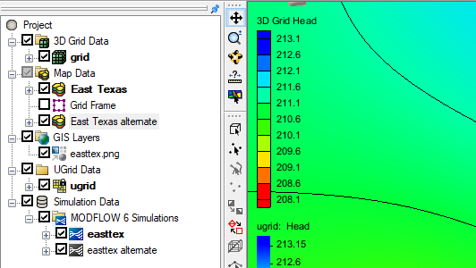
- You might find it useful to name each new project element with a name that helps describe it. Descriptive names can help you find your project elements more quickly when you need to tweak something here or there. For example, you might have a materials coverage where the default Manning’s n is 0.015 and another one where you’ve changed it to 0.045. Labeling the materials coverage “n-0.015” and “n-0.045” could help you remember the difference between the coverages.
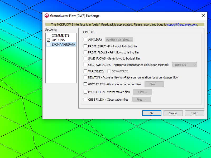
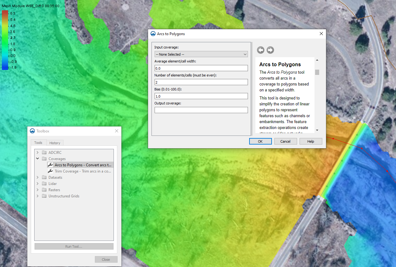
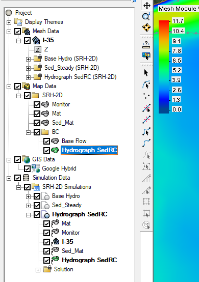
- You can add folders to organize items in the Project Explorer. For instance, you could group coverages according to which simulation you intend on using them for. Or maybe you have already imported a couple of rasters that you only need for one element of your project. You could put them together in a folder and collapse the folder in the Project Explorer. This will keep them out of sight while you don’t need them and could help you find them faster once you do need them. Note that solution data is automatically organized in folders in coordination with each simulation in the project.
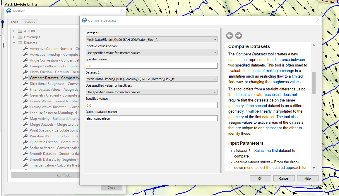
- You can add notes to most elements of your project. To add a note, use the Properties… right-click command on an item in the Project Explorer and go to the Notes tab. There, you can leave notes for your colleagues (or yourself) about the item’s intended use or provide additional information that is not readily apparent. This is particularly helpful with simulations when you can add a note giving a summary of the key features of that simulation. Notes could also be used to indicate datasets you compared to get a new dataset. These can help everyone keep track of what function each thing serves in a given project.
- As you go through the project, it is recommended to delete what you’re not using. Not only does this organize the Project Explorer, it also frees up space in SMS. This can help you avoid slow processing time that can come from too many simulations. In general, we recommend you not have more than seven simulations in a project. It is also recommended to remove large rasters, shapefiles, or images after you are done using them. If you want to keep certain elements that you’re not using right now, you may want to minimize them or put them in a folder when not in use.
Using these tips, you will keep your projects organized and accessible. Make use of the organization tools for the Project Explorer in SMS today!.