Aquaveo & Water Resources Engineering News

Transferring Data between GMS and ArcGIS Pro

Exporting and importing data between ArcGIS Pro and GMS allows many users to improve the quality of their groundwater models. Today we explore moving data between these two applications, focusing mostly on shapefiles.

Exporting and importing shapefiles allows features that have already been digitized in one program to be transferred to another program. For instance, once data has been modeled in GMS, it can be converted to a shapefile and imported into ArcGIS Pro. Furthermore, feature objects that have already been drawn in ArcGIS Pro or GMS can be transferred to the other program and then used as feature objects for the work you’re doing there.

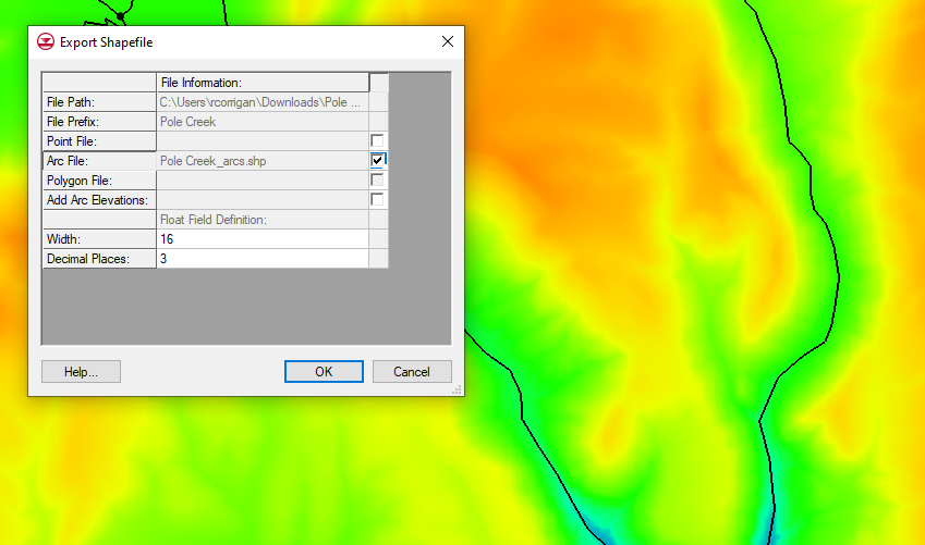
To start, consider exporting feature objects from GMS as a shapefile. You can draw arcs in a coverage and then use the right-click menu in the Project Explorer to export the information. There are three options for file type, so make sure to select "Shapefile (*.shp)" from the Save as type drop-down. Once you click Save in the Export Coverage dialog, another dialog opens that allows you to choose what kinds of shapefiles you want to save. There are arc, point, and polygon shapefiles. Once you've exported the shapefiles, they can be imported into ArcGIS Pro using that program’s Add Data function on the Map ribbon tab.

Exporting a shapefile from GMS

It's important to keep in mind that when GMS feature objects get exported to a shapefile, there are a couple of other file types that get exported with them. It's important to keep all of the files together because the shapefile is not complete without those other files. For example, one of the file types has projection information that lets other GIS programs, like ArcGIS Pro, know where the shapefile is located geographically. Without it, the shapefile is not attached to specific geographic coordinates, making it far less useful. You might consider putting all the files created in the shapefile together in a folder. This could help keep them together if you choose to relocate them after creating them.

GMS also allows for exporting of contour features and MODPATH particle tracking lines as shapefiles. However, these shapefiles do not appear when they are imported into ArcGIS Pro. Fortunately, there is a workaround for this issue. The shapefiles that GMS creates can be imported back into GMS after being exported. Then you can convert them to feature objects. Once they are converted to feature objects, you can use the same process described above to turn them into shapefiles that ArcGIS Pro can visualize.

GMS also has the ability to import shapefiles created or edited in ArcGIS Pro. Points, arcs, or polygons can be created in GMS, exported to ArcGIS Pro, edited in ArcGIS Pro, then saved and subsequently imported back into GMS. ArcGIS Pro also has exporting tools that can create shapefiles, CAD data, or other types of data for GMS to import.

There are other kinds of information that can be exported and imported between the two programs. Both programs have means for exporting and importing text files; 2D UGrids and other geometries in GMS can be exported as shapefiles; Rasters, scatter datasets, and other forms of data can also be transferred between GMS and ArcGIS Pro. In short, importing and exporting between these two programs has many possibilities.

Explore exporting and importing tools in GMS today!

Blog tags: 

Importing Data into CityWater

Do you have a project you want to import into CityWater? CityWater manages water distribution network models across local areas. Furthermore it empowers organizations to allow accessing and viewing of projects by multiple users.

A Citywater project is based on an initial project created in EPANET or Aquaveo's Watershed Modeling System (WMS). Once you have an EPANET project, you can upload it to the CityWater site. Currently, CityWater only accepts EPANET INP files. If you need to, you can download an EPANET application to convert a file to an INP file. Uploading may take some time depending on multiple factors such as:

  • The size of the file being uploaded
  • The availability of the server
  • The complexity of the area modeled in the file
  • Including fire flow options with the import

Uploading can range anywhere from less than a minute to twenty minutes or longer.

Processing status for CityWater INP import

Note that you cannot edit your uploaded file once it has been uploaded into CityWater. Any changes that need to be made to the model will need to be made in EPANET or Aquaveo's WMS application. It is strongly encouraged to review the INP file before importing it into CityWater.

If you have discovered that the imported project either needs changes or did not import correctly, you will likely need to delete the entire project, start over, and reupload the newly changed project. For this reason, we recommend that you review the project after it finishes uploading, before proceeding with using the tools in CityWater.

If the project file failed to import into CityWater, it could for a few different reasons:

  • There was an issue communicating with the server
  • The file is not a recognized file type
  • There is an issue with the CityWater new project parameters
  • There is an issue with the INP file
  • There is an issue with the EPANET project design

In most cases, these issues can be resolved by reviewing the INP file and attempting to import the file again. Try importing your EPANET file to CityWater today!

Blog tags: 

Organizing Project Files in SMS 13.2

Like most other data in Windows, SMS project files save into a directory that can be accessed via the Windows File Explorer. In SMS 13.2, the main project file gets saved with the ".sms" extension and most of the data and model information gets saved inside folders that appear alongside this main project file. The SMS file depends on those other files for the information about the project, and it will be incomplete without them. Comparison of file organization between SMS 13.2 and SMS 13.1

The names of the folders that appear next to the SMS project file depend on what kind of model is being built in SMS. For example, when an SRH-2D simulation is saved, a folder appears next to the SMS project file titled with the name of the tutorial followed by "_models." Additionally, some model will create an additional model folder with necessary components. For example, if a TUFLOW model is saved in the project, a folder named "TUFLOW" appears. For every SMS project file created by SMS 13.2, there is a folder created alongside it that starts with the name of the tutorial and ends with "_data".

The project folder needs every file created alongside it in order to be complete. This means it's essential to move all the files relevant to the project at once. SMS has a feature that "packages" the entire project for you. This feature facilitates keeping the files together when transferring the project to a different computer or a different user. To use this feature, select the File | Save As Package command in SMS. It puts all the contents of the project into a ZIP file that can then be moved to another location. When the ZIP file is unzipped in a different location, all of the necessary components for the project will be present and ready to use.

Now, while most of the data gets saved in two folders alongside the project, there are some files that get saved outside of those folders in the same folder as the project itself. If you are going to move the project without saving it as a package first, then remember to move every file pertinent to the package to the new location. We recommend saving each project in a separate folder to keep clear what information is relevant to a particular project.

It needs to be noted that when you are saving SMS files, the Windows character path length limit of 256 characters will apply. In order to make certain that SMS can access component files and subfolders for a project, SMS has a 150 character limit for the path length. This includes both the character in the project file name and the character of all folders leading to the project file.

Check out the project file organization in SMS 13.2 today!

Blog tags: 

Using Layer Range Options in GMS

The conceptual model approach in GMS is a very useful way to assign specific attributes to a MODFLOW model without having to manually input them cell by cell. One particularly helpful tool available in a GMS coverage is the "Layer Range" option.

Example of the Coverage Setup for Layer Ranges

Layer range can be used in addition to other coverage choices—such as streams, wells, rivers, head boundary, etc.—allowing you to be as precise as you need to be when applying your model attributes.

In the past, we have mentioned this tool in a blog post about assigning Ugrid attributes to specific layers, but that is only one of many helpful ways to use it. Here, we will go over each of the options available with the Layer Range, and exactly how they work.

First, turn on this option by selecting "Layer Range" in the sources/sinks column of the coverage setup dialog. At the bottom of this dialog, make sure that the default layer range for the coverage covers all the parts of your grid that you wish to use.

Second, apply feature objects to your coverage. In our example, we have created a Time-Variant Specified Head arc.

Example of the Layer Range Assignment in GMS

Once your feature objects are in place, you can assign values to them in the attribute table. This is where the Layer Range settings will come into play.

  • Use Layer Range: This option applies your feature objects to a specific range of layers. That range is selected in the attribute table under "From Layer" and "To Layer". A feature point assigned a layer range of 2–6 will be applied to every cell in that vertical column from layer 2 to layer 6.
    Similarly, a polygon or arc will apply its attributes to the whole assigned layer range for every vertical column that it intersects.
  • Auto-Assign BC to One Cell: Any time you want only one cell per column, you can choose "Auto-Assign BC to One Cell". This setting is especially useful when mapping an object type that can't or shouldn't be applied to more than one vertical cell at a time. Stream arcs are one example.
    Auto-assigning to one cell will use the elevation inputs from your feature object to choose the most applicable cell in that vertical column to receive the assigned attributes.
  • Auto-Assign BC Including Lower Cells: This setting allows the coverage to automatically calculate which initial layer the object is applicable to, similar to the "One Cell" option. It then applies the object to that cell, and to everything below it within the range of the coverage.
    Including the lower cells is very useful when you do want more than one vertical cell to be assigned, but need different layer ranges for different parts of the same feature object.

Once you have selected the Layer Range option that best suits your model, you can map the coverage to your simulation. The results can be viewed in the MODFLOW | Optional Packages dialogs, as well as the Sources/Sinks table in the right-click menu for the grid cells.

The Layer Range tool is a great way to get your model attributes as specific as you need them to be without any laborious manual editing. Try it out in your GMS model today.

Blog tags: