Aquaveo & Water Resources Engineering News

4 New Features in the WMS 11.0 Beta

For the last couple years, we’ve been working hard on the next version of WMS, and the beta for version 11.0 has now been released!

To help you learn about some of the new features, we’ve compiled this list of four new features in WMS 11.0 Beta.

  1. The first big improvement is a streamlined and updated set of floodplain delineation tools. Due to a lot of under-the-hood work, some of the delineation processes have been sped up by a factor of 10! This can greatly reduce the amount of time you spend on these projects.
  2. WMS 11.0 Beta now supports Amazon Terrain Tiles. These are high resolution digital elevation model (DEM) tiles for every location around the world, and the resolution goes as high as 3 meters per pixel. A digital elevation model is simply a two-dimensional array of elevation points with a constant x and y spacing.These DEM tiles can be accessed through the Import from Web and Get Data tools in WMS.
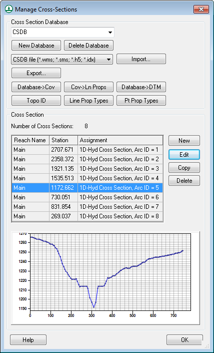
  3. Through a new dialog, WMS 11.0 Beta now offers better support for managing and editing cross section databases in HEC-RAS models. HEC-RAS is a one-dimensional model for computing water surface profiles for steady state or gradually varied flow. You can select, import, export, manage, and edit cross sections and cross section databases more easily.
  4. The hydraulic modeling module has been updated to be able to import and export LANDXML files for the Storm Water Management Model (SWMM), HY-12 (a storm drain analysis program used for designing inlets, pipes, and general storm drain network layouts), and EPANET (a widely used water distribution model developed by the US Environmental Protection Agency).

These are only some of the many great new and updated features in WMS 11.0 Beta. You can find a bigger list of them here. Try out the beta by downloading it today!

Blog tags: 

Converting Units

Seeing which units are being used in a project or for a particular object within the project is fairly easy. Converting the units from, for example, U.S. feet to meters, can introduce problems into a project if you do not do it in the correct way.

Reproject

Reprojecting the data involves moving the data from one coordinate system to another. So if your data is in a UTM coordinate system in meters and the rest of your project is in a State Plane projection that uses U.S. survey feet, reprojecting can change the data to match. Conceptually, the data will remain in the same location, but the data will be adjusted to the new units.

To reproject a dataset:

  1. Right-click on the dataset in the Project Explorer and select Reproject.
  2. In the Reproject dialog, the current projection is shown on the left. On the right side, set the new projection and units.

When converting units through reprojection, keep in mind that Z values (elevations) don’t always convert correctly. Round off errors sometimes occur when reprojecting data. In general, reproject does well in changing the X and Y units. The Z value, if it has been set as the bathymetry, typically also converts units well using the reproject option. Other datasets often do not convert between units using the reproject method.

When converting from rasters to scatter sets, the elevation is usually recognized and converted correctly.

Dataset Calculator

Datasets units can be converted using the Dataset Calculator. This is often necessary when the data has been reprojected, but not all of the datasets can be converted using that method. For example, a velocity dataset or conductivity data.

To convert a dataset with the Dataset Calculator:

  1. Select the desired dataset in the Project Explorer.
  2. Select the Data Calculator macro, or the Data Calculator command or the Dataset Toolbox command in the Data menu.
  3. Select the dataset to convert, then multiple or divide the dataset by the conversion value.

There are a few numbers it is useful to have when doing these conversions:

  • 0.304800609601 meters is equal to one U.S. Survey foot
  • 3.28083333333 U.S. Survey feet are equal to one meter
  • 0.3048 meters is equal to one International foot
  • 3.28083989501 International feet are equal to one meter

Note that there are many datasets that will not work with the Data Calculator.

In the end, make certain all the data being used in your model is in the correct units. Having mismatched units will typically create model errors and generate inaccurate results.

Try reprojecting data or using the Data Calculator to convert units in GMS, SMS, or WMS today!
Blog tags: 

Converting an RMA2 Project to SRH-2D

Do you have an older RMA2 or FESWMS project that you want to convert to an SRH-2D project in SMS? Older model lack the support and many of the features of newer models. In some cases, older models will no longer run with newer operating systems. So converting older projects over helps ensure the accuracy and stability of your results.

Converting projects from an older model is not automatic. Typically, portions of the model will need to be rebuilt. Here is an example of how to convert an older RMA2 model to an SRH-2D model.

Start with creating the SRH-2D mesh.

  1. Load the RMA2 project into the current version of SMS.
  2. Right-click on the RMA2 mesh, and select Duplicate. The duplicated mesh will be used for SRH-2D. The existing RMA2 mesh will be needed, so do not delete it.
  3. Select the duplicated mesh to make it active.
  4. Select the Data | Switch Current Model menu command.
  5. In the Select Current Model dialog, select the Generic Mesh option. The is the mesh type that SRH-2D supports. Be careful to not confuse the Generic Mesh option with the Generic Model option.
  6. Click Yes when warned that there may be data loss.
  7. Click Yes when warned that you are changing from a quadratic mesh to a linear mesh.

Next, you’ll need to define the boundary conditions.

  1. Select the RMA2 mesh to make it active.
  2. Select the Data | Mesh → Map menu command.
  3. In the Mesh → Map dialog, select the Nodestrings → Arc options.
  4. Select the Create New Coverage button.
  5. In the New Coverage dialog, select SRH-2D Boundary Conditions for the Coverage Type.
  6. When done, a new coverage will appear in the Project Explorer with feature arcs in the location of the nodestrings from the RMA2 project.
  7. Select each feature arc in turn and set boundary condition parameters that approximate those in the RMA2 model. Review the RMA2 boundary conditions if needed. Additional boundary conditions can also be added if desired.

You need to define the materials next.

  1. Select the RMA2 mesh to make it active.
  2. Select the Data | Mesh → Map menu command.
  3. In the Mesh → Map dialog, select the Material Regions → Polygons options.
  4. Select the Create New Coverage button.
  5. In the New Coverage dialog, select SRH-2D Materials for the Coverage Type.
  6. When done, a new coverage will appear the Project Explorer with polygons on the assigned materials in the RMA2 project.
  7. Review the material properties and the assigned materials for each polygon to make certain they converted correctly.

Finally, build the SRH-2D model simulation.

  1. Right-click in an empty space in the Project Explorer and select New Simulation | SRH-2D
  2. Link the SRH-2D mesh, boundary condition coverage, and material coverage to the new simulation.
  3. Right-click on the new simulation and select Model Control.
  4. Set the SRH-2D model control to approximate the conditions in the RMA2 model. Review the RMA2 model control if needed.

At this point, the RMA2 mesh could be removed and the SRH-2D model should be ready to run, though some tweaking may be necessary. Refer to the SRH-2D Troubleshooting Guide if needed.

Converting other models, such as FESWMS, follow a similar process to that described above. Try out this conversion process with your older projects today in SMS.

Blog tags: 

Using Mass Flux Computations

Are you wanting to compute the mass flux for a group of MODFLOW boundary conditions? The mass flux is the rate of mass flow per unit area, or mass per time per area. Computing this can quantify the strength of contaminants at a particular location in your model.

Use the MT3DMS or MT3D-USGS model to compute the mass flux at specific location. To do this:

  1. First create and run a MODFLOW model.
  2. Then create an MT3DMS or MT3D-USGS simulation with all relevant parameters set and contaminant species defined.
  3. Make certain the Transportation Observation Package is turned on in the MT3DMS/RT3D Packages dialog.
  4. If it is not already in the model, create a conceptual model with the MT3DMS/MT3D-USGS defined species.
  5. Create a map coverage with the observation point option for the species turned on.
  6. Create points on the coverage at the locations where you want to to observe mass flux.
  7. Assign these points as observation points and enter attributes as needed.
  8. Access the Transport Observation Package dialog through the MT3DMS or MT3D-USGS menu.
  9. Turn on the Compute mass flux at source/sinks option.
  10. Run the model.

MT3MDS/MT3D-USGS will compute the mass flux at each observation point. The computation is done using the units set for the input concentration. Typically, these are the units used for the display projection in GMS. So if your project is using U.S. survey feet, then your mass flux will be calculated as ft^3*mg/L. If varying units are used in the concentrations, then conversions must be done before calculating the mass flux.

The mass flux will be contained in a dataset file with the “.mfx” file extension. This file can be opened using any text editor. The file will show the calculated mass flux for each time step and for each source or sink included in the model.

Hopefully, you now understand a little more about calculating mass flux in GMS. Try out mass flux calculations and other features in GMS today!

Blog tags: 

Visualizing Meteorological Data

Do have rainfall data you would like to visualize in WMS? Inside WMS there are a couple tools to make your rainfall data visually interesting.

After you have imported your precipitation data, such as NEXRAD data, you can adjust your display options and/or create an animation.

Adjusting the Display Options

  1. Use the Display | Display Options command to open the Display Options dialog.
  2. Adjust your display options to show the data you want captured. It is recommended to turn on the Contours options.
  3. If using the Contours option, right-click on your rainfall dataset under 2D Grid Data and select Contour Options to open the Contour Options dialog.
  4. Adjust the contour method and interval to best display your rainfall data.
  5. With the down arrow key on the keyboard, step through the time steps in the properties window on the right sidebar to see how the precipitation varies.

Creating an Animation Loop

  1. Select your rainfall dataset in the 2-D Grid Module. The selected dataset will be used to create the film loop and can be cumulative or incremental. View incremental rainfall datasets in the same way as cumulative datasets.
  2. Select the Data | Film Loop command to open the Film Loop Setup Wizard. This wizard needs to be opened with the 2-D Grid Module active in order to have access to the meteorological data options.
  3. The first step in the Film Loop Setup wizard is essentially the same as creating any other animation through WMS. Select the location where the animation file will be saved and the type of film loop to generate.
  4. The second step of the Film Loop Setup wizard is to set the desired time step options for the rainfall data.
  5. The final step is where you will finalize the display options of the animation, and click Finish.
  6. WMS will take a few moments to create and save the animation file. The animation will start playing as soon as the saving process is complete.

When all is done, you can view your animation using the AVI play provided with the WMS installation, or you can use another application, such as GoogleEarth. The animation will display the movement of the storm through the selected time steps.

Try visualizing meteorological data in WMS today!

Blog tags: