Aquaveo & Water Resources Engineering News

How to Export Contour Lines as Shapefiles in SMS

Have you been wanting to export the contour lines in your SMS project as a shapefile so they can be opened in a different application? SMS allows exporting contour lines as a shapefile. This post will explain how to export contour lines as shapefiles.

Saving your contours as a shapefile requires your project to be set up correctly. Save the contours as a shapefile by doing the following:

  1. Make sure the contours you want to convert to a shapefile are set to Linear in the Display Options. To do so, open Display Options and click on the page for the geometry that has the contoured dataset loaded (e.g. mesh, UGrid, etc.). First, make sure that contours are turned on. Then, click on the Contours tab. In the Contour Method in the top left, make certain the first dropdown is set to "Linear".
  2. Make sure the desired dataset is active in SMS. This can be done by clicking on the dataset in the Project Explorer.
  3. In the File menu, select the Save As command. In the Save as type drop-down menu, select Shapes Files (*.shp). Then navigate to the desired directory. Make sure it's somewhere you will know how to find it. Then click Save.
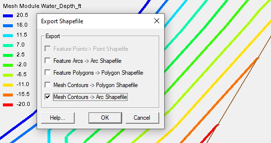
  4. Once you’ve clicked Save, a dialog opens that gives you options for converting project information to a shapefile. Select one of the contour options. The “Mesh Contours → Arc Shapefile” option is usually best.
  5. Now open your shapefile in the appropriate GIS software. The contour lines will appear as arc lines.
Example of Exporting a Shapefile from SMS

If you encounter issues with the shapefile, start by checking the folder where you saved the file. Make certain that all of the necessary files for the shapefile are there, including a projection file.

Another item to check is that everything you want in the shapefile is displayed correctly in the Graphics Window before you export. Try using the Uncheck All command in the Project Explorer and then checking only the desired geometry. This could allow you to more clearly see the contours as they will appear in the shapefile. You might also consider using the display options to turn off the geometry elements. This would also allow for clearer visualization of the contours. Once you can see the contour lines clearly, use the display options to adjust the contour lines if needed. Finally, there may be some differences between how SMS displays a shapefile and how other GIS applications display the shapefile. Opening the shapefile in SMS can help you determine if this is the case.

Be aware that selecting the Mesh Contours → Polygon Shapefile option when exporting the shapefile causes SMS to create a shapefile with only polygons. This might not accurately reflect the linear contours displayed in SMS since some of them might be only line segments.

Try out exporting contour lines as shapefiles in SMS today!

Blog tags: 

Risk Analysis for Well Groups

In your groundwater model, do you need a way to capture multiple wells for risk analysis? For example, your project might have multiple pumping wells and you would like to see the probabilistic composite capture zone for all wells in the wellfield. GMS provides a way to access the Risk Analysis dialog for refining stochastic modeling results.

Example of the Risk Analysis Wizard in GMS
  1. First open your project in GMS, making sure to select the Plan View and 3D grid module, it will be more difficult to select wells otherwise.
  2. Using the Select Cells tool, drag a box around the entire grid to select all cells in the grid.
  3. Open the 3D Grid Cell Properties dialog and change the value for the MODPATH zone code to a number of your choice.
  4. Select the coverage of the well to make it active. Using the Select Points/Nodes tool, drag a box around the entire project to select all wells in the coverage.
  5. Select Intersecting Objects to open the Select Objects of Type dialog.
  6. Select 3D grid cells from the list and close the dialog. This will select all 3D grid cells that have a well in them.
  7. Open the 3D Grid Cell Properties dialog.
  8. Change the value for the MODPATH zone code to a different number than the one that was used before, close the dialog and save changes. From here, the probabilistic capture zone analysis should be able to run with the well groups setting turned on.

Please note that particles need to leave their original zone to be mapped on the risk analysis results. That is why nothing will show up when all cells were assigned to the same zone. The recommended solution is to change the zone code of just the cells with a well so that as many particles as possible can leave the assigned area.

GMS allows you to be as general or specific as you need when selecting wells for risk analysis. Try out using risk analysis for well groups using GMS today!

Blog tags: 

Hardware Guidance for XMS

Are you wondering about what computer system to use with GMS, SMS, or WMS (collectively known as XMS) to get the best performance? The hardware you select will certainly make a difference in how XMS performs. This blog post intends to give some guidance for selecting hardware for use with XMS.

What hardware is required will depend very much on which models you choose to run and how large the projects are. Many lower power systems will technically run the software, but the interface may be slow and the simulation may take a very long time to run. In the end, the computer components you choose will depend on what you intend to do and the budget you have to work with. To help in the decision-making process, we have included some recommendations and explanations on how different components will affect the performance of the software. Look at your budget and see what is reasonable; it is recommended that you get the best you can afford.

Example of System Hardware for XMS

For some basic system requirements, you can check out this page on our wiki. Note that these requirements will change over time as technology evolves. The system requirements will change as future advancements are implemented into XMS.

The CPU is the component that will make the most difference in how fast the software runs. When comparing CPUs, we recommend looking at single-core rather than multi-core performance. The reason for this is that many of the models in our software do not take full advantage of multiple CPU cores at the same time. That being said, we do recommend that the CPU have at least 4 cores to give everything the power that it needs. Remember that it should be the best that you can afford

For RAM, 16 GB is usually sufficient, but some very large projects have required more. You may also want to get more RAM if you plan to have more than one project open at the same time. Our office computers have 16-32 GB of RAM, depending on the machine.

For a graphics card, we recommend getting a current low to mid-range dedicated card designed for gaming. Large projects can require multiple gigabytes of VRAM, but our cards with 4GB have yet to run into issues needing more. The speed of the GPU will particularly affect how smoothly the pan, zoom, and rotate tools work.

For storage, we usually recommend having an SSD with plenty of space. Projects can end up taking quite a bit of disk space, especially if the Save As function is used frequently. Having faster storage will reduce project load times and how long it takes to save a project. Note that storing projects on external/network drives have been known to cause issues, so we recommend storing any project files you plan to open on a local drive. Again, it is recommended that you get the best you can afford.

Having the right hardware will increase the usefulness of XMS for your modeling projects. Check out the XMS software applications today!

Blog tags: 

Specifying Arc Lengths in SMS 13.2

Imagine yourself trying to get an arc in an SMS map coverage just the right length. You keep on moving around the endpoint, but that often moves its azimuth as well. What’s more, measuring the arc would require using the Measure tool, and maybe that’s not precise enough for you. Fortunately, the most recent release of SMS has a solution. Today, we take a closer look at the Specify Arc Length tool, a tool designed for helping you be detailed in creating arcs. This tool, which was released as part of the beta of SMS 13.2, enables you to extend or shorten an arc by a specified length.

Let’s say that you have drawn an arc, and it’s pretty close to what you wanted, but you would prefer it just a little longer. You could manually adjust it, but using the Specify Arc Length tool, you can make it exactly the length you prefer.

Here’s how:

  1. In the Map module, select the Select Feature Arc tool.
  2. Select the arc you want to modify.
  3. Right-click and select the Specify Arc Length command.
  4. In the Specify Arc Length dialog, specify the desired arc length in the New Arc Length section.
Example of the Specify Arc Length in SMS

If the desired arc length is longer than arc’s current length, then the arc extends to match the entered length. If the desired arc length is shorter than the arc’s current length, then a new node is created to shorten the arc. Shortening an arc results in the creation of two arcs.

There are some important things to keep in mind when using this new tool.

First, the arc can only be adjusted relative to the arc direction, which is usually the direction the arc was drawn (e.g. right to left) when it was created. This means extending the arc moves the end node of the arc in a straight line in the arc direction until the whole arc is the desired length. Shortening the arc adds a node the specified distance along the arc in the arc direction. This can be seen in the image below. The beginning of the arc (usually the node drawn first) never moves as a result of the Specify Arc Length tool.

It’s also important to be aware of the arcs attached to the arc you’re modifying. If the arc is attached to another arc, then extending the arc also modifies the length of the arc it is attached to. Be sure that adjusting both arc lengths is desirable before using this tool.

Furthermore, when extending an arc with many segments, note that only the segment at the end of the arc gets extended. The final segment extends in a straight line as shown below until the arc is the specified length. The rest of the segments are left untouched.

This is just one of the many tools that SMS13.2 makes available to enhance your water modeling capabilities. Try out using the Specify Arc Length tool in SMS 13.2 today.

Blog tags: 

Adding Multiple Screens to Well Points

Do you have multiple screens to add to your MNW2 wells? Adding multiple well screens can be an important part of modeling what a well situation looks like in real life. But you might be frustrated trying to figure out how to get multiple screens on your well points. Today, we detail how to add multiple screens on MNW2 wells.

While wells with singular screens can be imported using the GMS import wizard, adding more than one screen to a well necessitates a different workflow.

To add multiple screens, add them one at a time to each well:

Example of setting multiple well screens
  1. Create a coverage with MNW2 wells enabled.
  2. Use your TXT or CSV file to add the well points to your coverage through the import wizard.
  3. Once the points are in GMS, right-click on that coverage and choose Attribute Table.
  4. Make sure that your Show dropdown is set to "all", so that each well point is visible.
  5. If needed, uncheck the checkbox in the Use screen column.
  6. In the column labeled Boreline, click on the ... to open up the z screen table for one of your points.
  7. In that table, you can list (or copy/paste) all of the well screen values applicable to that well point.
  8. Repeat steps 5–7 for each well.

Since adding multiple screens is a manual task, staying organized is an important part of it. Consider keeping track of which wells you have already added screens to. You could keep track in a spreadsheet or in a notes application of your choice. This is especially important with a large number of wells because it is not obvious in the Attribute Table which wells already have screens assigned to them.

Again, adding multiple screens is specifically for MNW2 wells. So, if you have multiple screens to add to your wells, then you might consider changing them to MNW2 wells. This would allow the wells to accommodate adding multiple screens.

If you have a project needing multiple well screens, use GMS today!

Blog tags: 

Rebuilding an SRH-2D Restart File

Have you ever needed to rebuild an SRH-2D restart file for a project you were working on? Perhaps you lost the restart file or maybe you made modifications to your mesh, so the restart file is no longer valid for the model you have. Regardless of the cause, rebuilding a restart file can be a vital step in completing the model you're working on.

To start rebuilding your restart file, see if you can do a dry run of your simulation:

Example of the SRH-2D Model Control Set to Use a Dry Run
  1. Right-click on the simulation in the Project Explorer and select Duplicate.
  2. This ensures that the original simulation is preserved if needed.
  3. In the newly-created simulation, right-click and select Model Control to open the Model Control dialog.
  4. In the dialog on the General tab, for the Initial Condition drop-down select "Dry".

Every run of SRH-2D creates restart files for the model. Initially, it creates a restart file for every time step as determined by the Output Frequency in the Model Control dialog. However, when the solution is loaded into SMS, the software only saves the restart file for the final time step. If a restart file for a different time step in the simulation is desired, then please complete the following before clicking Load Solution in the Simulation Run Queue dialog:

  1. Browse to where the project is saved.
  2. Double-click on the folder with the same name as the SMS project.
  3. Double-click on the SRH-2D folder.
  4. Double-click on the folder with the same name as the simulation run.
  5. This is where restart files were written for every time step. The file that ends in "_TSO.dat" is a text file with information about which restart files correspond to each time step. Open it in a program that can read plain text files to make sure that you select the restart file with the desired time step. The restart files end in "_RST" followed by the time step number (e.g. "Standard_Run_RST12.dat").
  6. Once you have determined the restart file you want to save, copy and paste it in a different folder on your hard drive.
  7. Then click Load Solution in SMS.

SMS loads the results into SMS and keeps only the restart file for the final time step. It's important to remember that changing anything in the mesh necessitates the creation of a new restart file. Restart files should only be used with a model that uses the exact same mesh as the simulation that generated the restart file. Using the restart file with a slightly modified mesh might yield inaccurate results.

SRH-2 with SMS provides powerful tools for surface-water modeling. Use SMS today!

Blog tags: 

Trimming and Extending Arcs in SMS 13.2 Beta

Do you have arcs in a project that you need to extend or trim to match another arc? For example, you may be modeling a bridge with two arcs to represent the bridge in SMS. If you want to make certain the two arcs are the same length, you will need to extend or trim one of the arcs. A new tool introduced in SMS 13.2 allows you to trim or extend the length of arcs to match the length of another arc. This article will discuss how to trim or extend arcs as well as the advantages of doing so.

To use the Trim/Extend tool, do the following:

  1. Select one arc and, holding down the Shift key, select another arc. It is important to take note of what arc IDs are selected, trimming or extending the wrong ones can cause problems in the model.
  2. Right-click and select the Extend or Trim Arc command to open the Trim/Extend Arc tool.
  3. In the tool, there are two different options: one to select the arc that will be extended or trimmed and another option to select which arc will be used as the base arc for the length.
Example of Trim/Extend Arc in SMS

There are a few ways to differentiate between wether you are extending or trimming an arc. With the extend option, the number of intersections included in the arc selection will indicate to the tool to use the "extend" operation. Whereas with the trim option, if one or more intersections are included in the selection, this indicates a "trim" operation. This will allow a node to be inserted into the first arc at the first intersection and delete the first portion of the newly split arc.

It should be noted that you can only select up to two arcs otherwise the option to trim or extend will not appear. Try trimming or extending arcs in SMS 13.2 beta today!

Blog tags: 

Using the UPW Package for MODLFOW-NWT

Do you have a groundwater model that might benefit from using the UPW package in GMS? The Upstream-Weighting (UPW) package is one of the four available options for flow packages for MODFLOW. It is used for calculating intercell conductances in a different manner than is done in the Block-Centered Flow (BCF), Layer Property Flow (LPF), or Hydrogeologic-Unit Flow (HUF) packages.Rather than the discrete approach of drying and rewetting that is used by the BCF, LPF, and HUF Packages, the UPW package treats nonlinearities of cell drying and rewetting by use of a continuous function of groundwater head.

Example of the UPW Package dialog

In order to use the UPW, you first need to have a MODFLOW-NWT simulation as part of your groundwater model in GMS. Once you have selected the MODFLOW-NWT version, you can use the Packages dialog to activate the UPW package.

The UPW flow package is based on the LPF package but differs in that the rewetting and vertical conductance correction options are not available. Otherwise, the UPW package allows you to work with both confined and convertible layers. It also has options for vertical hydraulic conductivity and interblock transmissivity. Array values can be set for the horizontal hydraulic conductivity, and vertical and horizontal anisotropy using the MODFLOW array editor in GMS.

Additional options are also included here. It is possible to remove vertical leakance correction or set a head value for dry cells. These options are in their own dialog accessible through the main UPW package dialog.

It should be noted that the UPW flow package is only available for use in the MODFLOW-NWT model and is not available with other versions of MODFLOW. The UPW is designed to work with the NWT linearization approach which generates an asymmetric matrix.

If you have a MODFLOW-NWT groundwater model that needs a different approach to calculating conductance, try out the UPW package in GMS today!

Blog tags: 

Curve Number Values for NLCD Land Use Data

Are you wondering what values to use for composite curve numbers used with NLCD land use data in your WMS project? WMS contains a Compute GIS Attributes calculator in the Hydrologic Modeling Module that allows you to import composite curve numbers to use in land use mapping. This can allow you to define boundaries for different soils, rainfall depths, etc. This post will cover some different resources to get the values you need.

Compute GIS Attributes with Imported Curve Data

It is important to be aware that there are two options when using the Computing GIS Attributes calculator: WMS Coverages as well as GIS Layers. With both GIS Layers and WMS Coverages you are given the option of selecting the Soil Layer Name, Drainage coverage computation step, etc. In the GIS Layers you are given the option to view field records and assign a code of your choosing. To use the GIS Layers option, you will need to have already imported GIS data into your project. In order to make the WMS Coverages option active you will need to have created your own land use or soil type coverages within WMS. Using the WMS Coverage option allows you to import your own land use or soil curve numbers from a text file.

What values you use for the text file depends on your own judgment and what would work best for your project. One option to get the table values is to use the example files found on XMS Wiki in the SCS Curve Numbers section. Opening one of these examples will show you an area-weighted average of the different curve numbers for the different regions. Another option is to visit the USGS website, download the example data, and import it into the GIS Attributes dialog. Finally, you can make your own table In which case use your engineering judgment to determine the CN values for your project.

Try out inserting curve number values for NLCD land use data in WMS today!

Blog tags: 

Merging Map Coverages in SMS

Do you have an SMS project that might benefit from merging coverages together? It’s not uncommon to have feature objects on different map coverages in SMS that would be useful to have on one coverage. For example, you might have feature objects from a shapefile on one coverage that you would like to merge with feature objects you have created on another coverage. This post will cover some tips to merge coverages as well as the effects of merging coverages.

To merge map coverages:

  1. Select one coverage in the Project Explorer then hold down the Ctrl key and select another coverage.
  2. Next right-click and the Merge Coverages command will appear.
  3. After clicking the Merge Coverage command, a warning dialog will ask you if you want to keep or delete the coverages being merged.
  4. Upon completion a new merged coverage will appear in the Project Explorer.
Example of Merging Map Coverages in SMS

Merging coverages comes with a lot of benefits when working with a large number of feature objects. When merging coverages here are a few items to keep in mind:

  • When merging coverages of different types, the new merged coverage will be converted to the Area Properties type.
  • When merging coverages of the same type, the new merged coverage will be the same type. For example, if you had two map coverages that are both ADCIRC materials they are going to remain ADCIRC Materials after they have been merged together.
  • When merging, only the feature objects will be merged together–any defined attributes on the feature objects will be reverted to the default setting for that coverage type. For example, the default for SRH-2D boundary conditions coverage type is the wall boundary condition. When two SRH-2D boundary condition coverages are merged all the arcs will be set to have the wall attributes.
  • When only wanting to copy a few feature objects from one coverage to another, use the Copy to Coverage feature instead of merging entire coverages.

These are just a few tips to help with merging coverages in SMS. Try out merging coverages in SMS 13.2 today!

Blog tags: 

Pages