Aquaveo & Water Resources Engineering News

Defining UGrids Layer Attributes in GMS

In your groundwater model, do you need to define MODFLOW-USG attributes for a UGrid that vary by layer? For example, you might have multiple polygons that define your recharge zones for your model where the attributes on each polygon are only meant to be applied to specific layers on the UGrid. GMS provides tools for specifying how those attribute definitions get applied to UGrids.

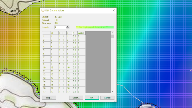
First, you can always apply attributes directly to a UGrid using the grid approach. Doing this has the advantage of having direct control over the attributes assigned to each cell and element on each layer. However, doing this on a large UGrid or for more complex models, this can become tedious and time consuming. Using the conceptual model can aid in managing assigning attributes to layers in more complex models.

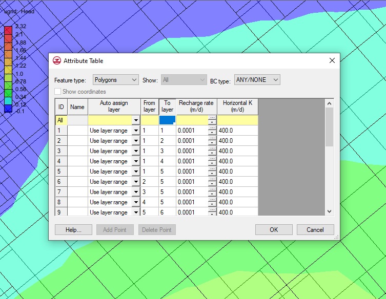
For the conceptual model approach, the Coverage Setup allows you to specify the layer range for sources, sinks, boundary conditions, and areal properties. The Layer range option must be turned on in order to specify the layer range for attributes applied to feature objects in the coverage. If Layer range option is not applied then the default layer range will be used when applying attributes on the coverage to the UGrid.

Example of Specified Layer Ranges in the Attribute Table

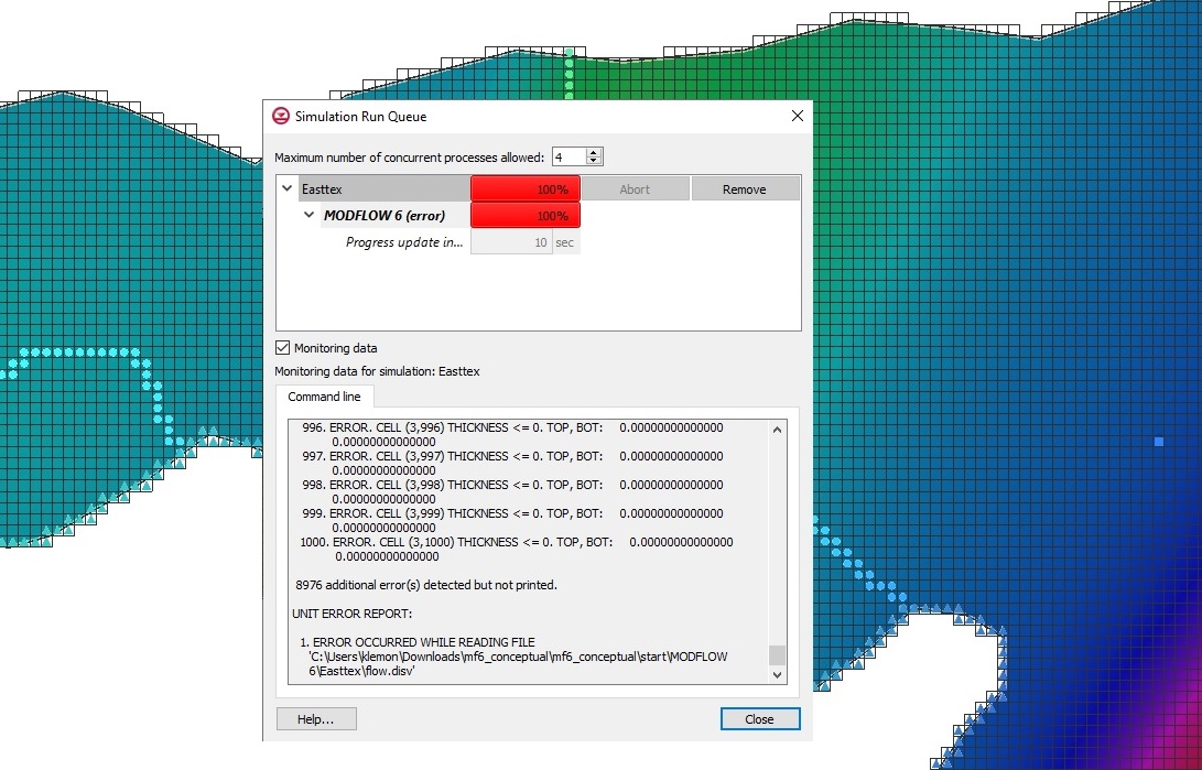
It should be noted that once you have chosen to assign attributes to specific layers, you will need to pay attention to which attributes are being assigned. It is recommended that you review the assigned MODFLOW attributes. Keep in mind that you cannot mix specified layer ranges with the default layer range. GMS does not give priority to the default layer range over the specified layer ranges and vice versa. For example, if you assign refinement attributes to a polygon to use a specific layer range, but leave other polygons on the same coverage to use the default layer range for refinement, this will likely cause issues in the model run or results.

GMS allows you to be as general or specific as you need when assigning MODFLOW attributes to UGrid layers. Try out defining the layer attributes for UGrids in GMS today!

Blog tags: 

Comparing SRH-2D and HEC-RAS Solutions

Have you ever wanted to compare model results between SRH-2D and HEC-RAS models? The SMS 13.2 interface allows you to view both SRH-2D and 2D HEC-RAS results for the same model at the same time.

Say, for instance, that you have created an SRH-2D simulation in SMS and you want to compare results using HEC-RAS. First, if you do not have the project in both SRH-2D and HEC-RAS, you will need to create an HEC-RAS simulation in SMS and use it to export the SRH-2D mesh into a file format that HEC-RAS can use. Then you can import the mesh into HEC-RAS and set up the boundary conditions and other attributes of the simulation.

Comparing a SRH-2D and HEC_RAS simualtion

Once you have a completed simulation for both SRH-2D and HEC-RAS, you can import the results of the HEC-RAS simulation into the SMS project containing the SRH-2D solution. To do this, simply open the "*.p**.hdf" file generated by HEC-RAS in SMS. This will import the HEC-RAS solution into your SMS project. The HEC-RAS simulation solution will appear on a 2D UGrid.

There are many different comparison options available, a few are listed below:

  • The first comparison is often a quick visual check. Switching between the two models in the Project Explorer will let you make quick visual comparisons. You may need to adjust your contour display options to make this easier.
  • Using the Data Calculator, you can make a comparison dataset. Since the HEC-RAS solution will be on a UGrid and the SHR-2D solution will be attached to a 2D mesh, you may need to convert data to be in the same module in order to do this.
  • Observation Plots are another way to compare the models. You can plot the solutions from both models using the same observation coverage.

Try out comparing SHR-2D and HEC-RAS models in SMS 13.2 today!

Blog tags: 

Exporting Map Coverages in SMS

Do you have a map coverage with specific defined attributes in an SMS project that you would like to add to another project? There is a solution: starting in SMS 13.2 you can export your map coverage as a DMC file that you can import into another project.

For exmaple, say that you have defined a weir structure on an SRH-2D boundary condition coverage for your project. You could, conceivably, have a massive project with many different coverages, meshes, and simulations. If you, or a coworker, would like to use that weir with its defined attributes in another project, recreating the same weir would be inefficient. Instead, exporting just the weir coverage as a DMC file allows you to import the weir coverage with its feature objects and attributes into another project. This will save time for everyone involved in the project, streamlining the process.

There are three steps to export a map DMC:

  1. Right-click on a coverage of your choice in the Project Explorer and select the Export command.
  2. In the Export Coverage dialog, change Save as type to be "SMS model coverage (*.dmc)".
  3. Save the DMC file.
Example of Exporting a Map Coverage as DMC File

The DMC file can now be imported into another project. Importing the DMC file will create a new map coverage in the project with all of the feature objects and attributes that were saved with the file.

It should be noted: Nearly all attributes in the coverage will be exported. The exception to this rule is that external files referenced by the coverage are not embedded in the model coverage file. An example of this would be an external tidal WSE source in a CMS-Flow BC coverage. The attribute would include the link to the file, but if the DMC file is read into a project on a different machine, the external file would not be in the same location, and therefore the association is automatically maintained.

It should also be noted that not all map coverage types can be exported as a DMC file. Certain older map coverage types do not have this option at this time.

Try exporting a DMC file and importing it into an SMS 13.2 project today!

Blog tags: 

Using the MODFLOW 6 Run Queue

Have you noticed that in GMS MODFLOW 6 uses a different model wrapper than other MODFLOW versions? This model wrapper is the SImulation Run Queue and it has a few new options. Since MOFLOW 6 in GMS allows having multiple simulations run, the Simulation Run Queue helps you manage the different simulation runs.

The new Simulation Run Queue dialog functions a little differently from the Model Wrapper dialog. Some of the changes include:

  • You must click Load Solution to load the desired simulation solution into the project. This does not happen automatically when you click close as it does with the MODFLOW model wrapper.
  • If you try to run a simulation already in the queue, you will be prompted to remove the simulation from the run queue before it can be run again.
  • If changing an active simulation’s settings, renaming the active simulation, or taking any action that affects a simulation currently in the queue, you will be asked to remove the simulation from the queue prior to making the changes.
  • The maximum number of concurrent processes allowed can be as many as you want. However, it should be noted that the more complicated the simulations the longer it may take for the processes to complete. Therefore, allowing a large number of processes to run concurrently may slow down processing time if you are running multiple complex simulations.
  • Turning on the Monitoring data will allow you to see the command line run for each process. This can be used to troubleshoot issues that may have occurred during the simulation run. If the simulation encounters an error look to the Command line to see what has caused the error. If there are no errors then your simulation should show 100% in green instead of red (denoting an error).
  • Another important note is that you can still work while the simulation is running. You can move the Simulation Run Queue to the side and continue to work on your project while it runs. Right-clicking on the simulation folder in the Project Explorer provides a command for opening the Simulation Run Queue if you accidentally close it.
Example an error in the MODFLOW 6 simualtion in the Simulation Run Queue

Now that you know a little more about the Simulation Run Queue dialog in GMS 10.6 try it out today!

Blog tags: 

Tips for Working with Virtual Machines

Have you installed GMS, SMS, or WMS (collectively referred to as XMS) on a virtual machine in your office? Using a virtual machine is often done in order to run multiple operating systems, consolidate computing resources, provide integrated disaster recovery, or a number of other reasons. XMS software can be installed on a virtual machine in order to fit your needs. Here are some tips for working with XMS when using a virtual machine.

Virutal machine

First, make certain that your XMS license is compatible with a virtual machine. Both local and flex license codes can be used with a virtual machine. However, local codes will not allow the software to be used by other machines. Older single-user locks cannot be used with a virtual machine.

When using a flex license, the virtual machine will need to have access to the local network in order for other machines to access the XMS license and use the software. Both the XMS application and the Aquaveo License manager need to be installed on the virtual machine.

When sharing files between a virtual machine and a host machine, pay attention to where XMS is running. XMS requires that all files be placed where XMS is installed. Therefore, you cannot save your project on the host machine and run them from the virtual machine if XMS is installed on the virtual machine. You will need to move the files to the virtual machine where XMS and XMS license is installed.

It should also be noted that some simulation runs and application processes in XMS will run slower on a virtual machine than running the same process directly on a physical machine. This is due to the nature of using a virtual machine. If there is a process that is taking an unusually long time, it is recommended that you try running the application on a physical machine.

If you are experiencing issues running XMS on a virtual machine, contact our technical support team and they will be happy to assist you.

Blog tags: 

Tips for Using ADCIRC with SMS

ADCIRC is a popular numeric model that works with the SMS graphical interface. The SMS interface adds a number of tools and features to improve and enhance the use of the ADCIRC model. When building an ADCIRC model in SMS, there are a few items to keep in mind. This article will review some of the best practices for building an ADCIRC model in SMS.

  1. When importing a fort.22 file, the ADCIRC control file must be imported to read the data in the fort.22 file. If the fort.22 happens to be a best track format file (NWS=8,19,20), add the ".atcf" extension to the file name so that SMS can import the file and create a wind track coverage. This is the only format of fort.22 that is independent enough of the fort.15 to reasonably expect anything to happen on import.
  2. It can be tempting to create an ADCIRC mesh in SMS, then manually edit the fort.14 file to fine-tune some aspects of the mesh/grid. This is not recommended. Doing this may cause the mesh to not be usable once imported into SMS. It may also cause certain functions to fail such as converting mesh features to a coverage or mapping tidal components. This is not always the case, but care should be taken when editing the fort.14 file outside of SMS. In general, it is not advisable. The model checker may catch these issues, but in some cases the model checker will miss the error.
  3. It is usually best to make certain that the mesh/grid has what you need before adding it to the simulation. Editing the mesh in SMS after it has been linked to a simulation may require that the mesh be unlinked and re-applied to the simulation.
  4. Older ADCIRC projects can be added to the most recent version of SMS. When doing this, SMS will convert and update the project. It is recommended that you review the project once it has been converted. Projects created in newer versions of SMS typically cannot be imported into older versions of SMS.
Example an ADCIRC project in SMS

For additional support in using ADCIRC with SMS, contact our technical support team at: support@aquaveo.com

ADCIRC and SMS gives you greater flexibility in coastal modeling. Try out ADCIRC with SMS today!

Blog tags: 

Running MODFLOW Outside of GMS

Do you have a MODFLOW project you created in GMS, but realize you need to run MODFLOW outside of GMS? This is sometimes necessary if you have a very specific need for your project that can only be accomplished by modifying the exported files before running the MODFLOW simulation. This does not happen often, but when you do encounter a situation where you need to run MODFLOW outside of GMS, do the following:

  1. Open the MODFLOW Global Options and make certain that the Save as Native Text option has been turned on. This is necessary to generate files for your project that you can edit. With the native text option turned on, saving your project will generate the native text files.
  2. One you have the native text files generated, you can then edit the files manually using a text editor. GMS will create a separate directory with the native MODFLOW files. This directory will typically be the project name with "_text" appended to it. For example, if the project is named "Aquifer", the directory will be named "Aquifer_text". Keep these files together.
  3. Running MODFLOW using the Command Prompt
  4. To run the native files, use either a command line with a DOS prompt or a batch file. See guidance for how to do this on USGS's website.
  5. After you have successfully run your MODFLOW simulation, import back into GMS to visualize the results and perform additional analyses using the tools in GMS. You will need to start by importing either the NAM file or MFN file. These files contain a directory for the other files in the MODFLOW project and how they should be opened. It is important to keep all of the MODFLOW files together in the same directory. Having only the NAME or MFN file will not be enough to open the MODFLOW project. Files for the packages used with the project will typically have a file extension that matches the package. For example, the Wells package will have the extension "*.wel".

Running the native files outside of GMS can be used to validate results of a GMS model or to add custom parameters not available in GMS. However, Aquaveo may not be able to provide technical support for simulations that have been extensively modified outside of the GMS application.

Knowing how to run MODFLOW outside of GMS can give you more options for modeling with GMS. Try out GMS 10.6 today!

Blog tags: 

Registering an Image in XMS

Do you have an image that you would like to add to your project, but that image doesn’t have any coordinate information? Many projects require that you have an image or map that defines the proposed location for structures, wells, or other objects. In XMS (GMS, SMS, and WMS) the image needs to have coordinate information in order to correctly align with the project data. If your image does not have coordinate information, the Register Image dialog will appear.

Example of the Register Image dialog

To use the Register Image dialog, designate three points on the image and enter the coordinate information for those points. XMS will then use those coordinates to create the coordinate data for the entire image. It is possible to register an image using only two points, but three points is recommended.

If you do not know the coordinate information for any points on the image, here is a tip for getting coordinate information for the image.

  1. Click the Add Online Maps macro to open the Virtual Earth Map Locator dialog.
  2. Search for the area of your image by putting the name into the search bar and click Jump to Search Location.
  3. Be sure that the entire project bounds are within the window and match the area of your unregistered image.
  4. Download the new image and set the projection for this image.
  5. Note: you could just use this new image, but if the image you are trying to import shows the location of proposed structures, boreholes, etc., then you may need to still import the unregistered image.
  6. Outside of XMS, use a photo viewer to open the unregistered image.
  7. Compare both images and find three places where you can easily tell that the images match up.
  8. Now, in XMS, place your mouse over one of the three locations that you will need the geographical coordinates for.
  9. At the bottom of XMS you can view the coordinate information. Write down the coordinate information, then repeat in two other places.
  10. Now that you have all of the location coordinates you need to register the image, open the unregistered image file in XMS to bring up the Register Image dialog.
  11. Click the three points you have coordinate information for and enter in the coordinates that you wrote down earlier.
  12. After registering the image, check the alignment of the images if needed.
  13. Try registering an image for your project in SMS, GMS, or WMS today!

Blog tags: 

Reducing Scour in SRH-2D Sediment Transport

Do you have an SRH-2D sediment transport model that has an unreasonable amount of scouring? There could be several different issues in your model that are causing unreasonable scouring, however, SMS contains several different ways to fix this issue. This article will cover how to limit scouring so it is put to extremes in your model.

  1. Review the sediment loading on your boundary conditions for the sediment transport model. Double-click on one of your boundaries to check your sediment boundary conditions to review how the sediment loading has been defined. In the SRH-2D Assign BC dialog check and update the Sediment inflow section if needed.
  2. Example of scouring within an SRH-2D sediment transport model. The image on top shows the scour and the lower image it has been fixed.
  3. For your sediment transport SRH-2D simulation, go to SRH-2D Model Control and select the Sediment tab. Review the Particle diameter threshold section to make certain that the sizes are reasonable. Often having diameters that are too large causes scouring.

  4. Another place to review is the SRh-2D sediment material coverage. Right-click on the click Materials List and Properties. Under Gradation Curve, right-click on one of the materials and select click Edit Curve to bring up the Gradation Curve dialog. Review the gradation values and check for inconsistencies. Remember that the values need to be scaled from the smallest sand to the largest boulder. It is important to remember that the maximum number of functioning rows only goes up to nine. Any more than this will cause inconsistencies to appear.

    When the values that are entered in the Sediment Gradation Parameters are put to extreme values this is what will often cause the deep scour you may see in your model. A regular model will be smooth with very little deviation. A helpful resource to use if things are still not clear is the USBR website. They have example problems that you can follow.

These are just some of the tips for reducing scouring in your SRH-2D sediment transport models. For additional support for sediment transport with SRH-2D contact our technical support team. Try out SRH-2D with sediment transport in SMS 13.2 today!

Blog tags: 

Exporting Using the View Values Command

In your groundwater model in GMS, do you need to export only a specific dataset value? GMS provides a way for you to export different dataset values and save them as text files that you can continue to edit outside of GMS. This post will cover exporting values using the View Values command.

To export data using the View Values command, select a dataset in the Project Explorer then right-click and select the View Values command. This will open the Edit Dataset Values dialog. This dialog shows an array of data values for the selected dataset. From the Edit Dataset Values dialog, you can export the data values in a couple ways.

Example of the Edit Dataset Values dialog

The first option is to click the Export button in the dialog. This will open the Dataset Filename dialog. Here you can give the exported file a name and save out the data as a tabular text formatted file. This exported file can be opened with a text editor or spreadsheet program. All values in the dataset will be exported with this value.

The second option is to select the data in the data array, then copy (Ctrl+C) and paste (Ctrl+V) the values into another document such as Excel or Google Docs. This method gives you the option to be selective about which data values to include. This method also allows you to save out the data in other file formats.

It is important to note that if you change the formatting in the text file, in excel, or google sheets and try to import the file back into GMS it may not import correctly. The format used in the Edit Dataset Values dialog is the format that GMS will be expecting when importing the data back into the project.

Try out exporting dataset values using the View Values command in GMS today!

Blog tags: 

Pages