Converting a Lidar File to a DEM in WMS
By aquaveo on June 2, 2021Do you have a lidar file that you would like to convert into a DEM file? WMS can help you with this. Lidar files can contain a large amount of 3D points used for representing features on the Earth’s surface. DEMs can be derived from high-resolution LIDAR data, and we have developed a workflow that can do this. This post will review how to convert LIDAR files to DEM files quickly and easily in WMS.
This can be done by using the following workflow:
- Use any of the methods to open files to import your lidar files into your WMS project.
- If you have more than one lidar file imported into the GIS module, select all of the separate files and then right-click one of them and select Merge… to open the Lidar File dialog where you can name and save your merged lidar file.
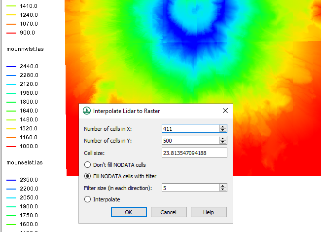
- After you have imported your lidar file, right-click it in the Project Explorer and select Interpolate to | Raster… to open the Interpolate Lidar to Raster dialog.
- Review the settings and click OK when they are all set correctly.
- In the Raster File dialog, set the name and type for the raster file and then click Save to close the dialog and save the raster file.
- When done generating the raster and updating the display, right-click the new raster file in the GIS module and select Convert to | DEM to open the Resample and Export Raster dialog.
- Review the settings and click OK when they are all set correctly.
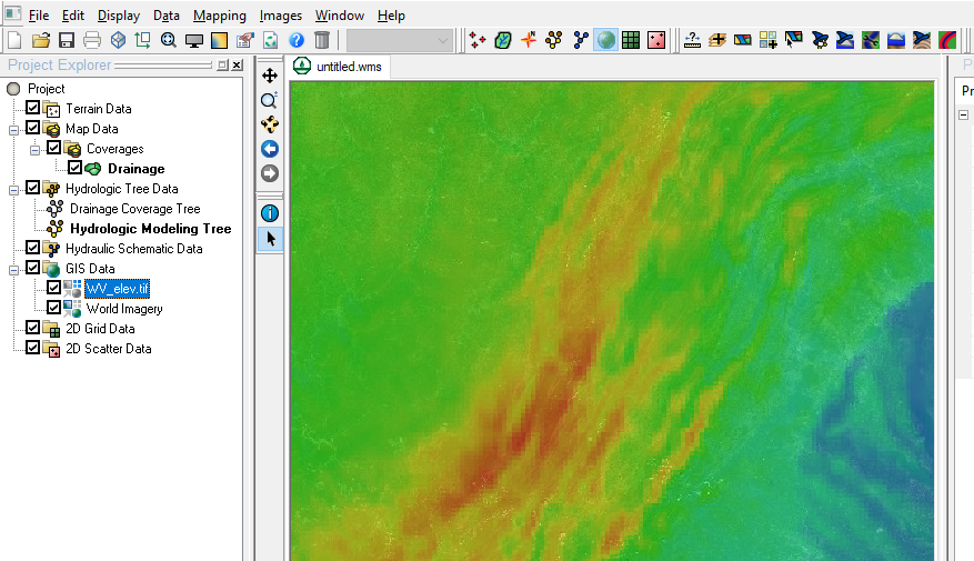
- You should now have a DEM file of the same area as your lidar files. Hide everything in the GIS module to view the DEM file on its own.
It should be noted that if you have multiple lidar files, you can convert each file individually rather than merging them all together as was done in Step 2. The merge makes the final product easier and quicker to accomplish.
Try out converting lidar files to DEMs in WMS today!