Viewing Vectors on the Watersurface
By aquaveo on August 19, 2020With the release of SMS 13.1 beta, a new option has been added to the Vector tab. The existing Vector tab in the Display Options dialog allows viewing vector data as arrows as data points in your project. SMS can change the density of how the vector arrows are displayed and to display the vector arrows along a constant elevation. This new option allows you to display the model vectors relative to a selected dataset.
To use this option:
- Open the Display Options, turn on vectors, and go to the Vector tab.
- On the Vector tab and change the Origin to be "Relative to dataset".
- Select the Dataset button under the Origin to bring a tree item selector dialog.
- Select the Dataset you want to use.
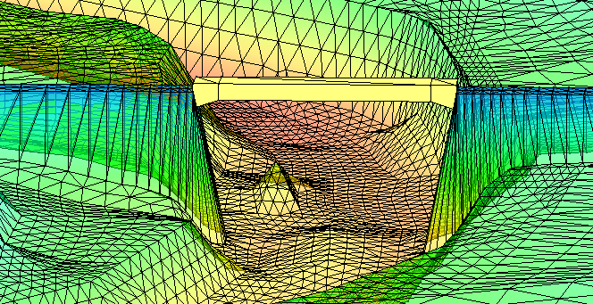
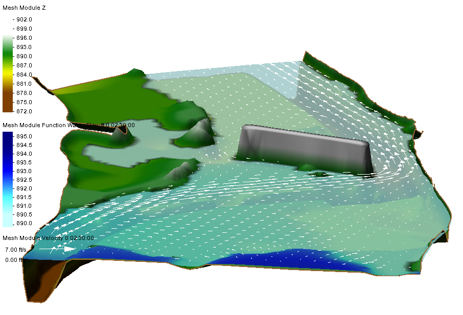
After closing out the Display Options dialog, you will be able to see the vectors relative to the selected dataset. For example, if you use a water surface elevation dataset, you would be able to see the vectors relative to the water surface elevation.
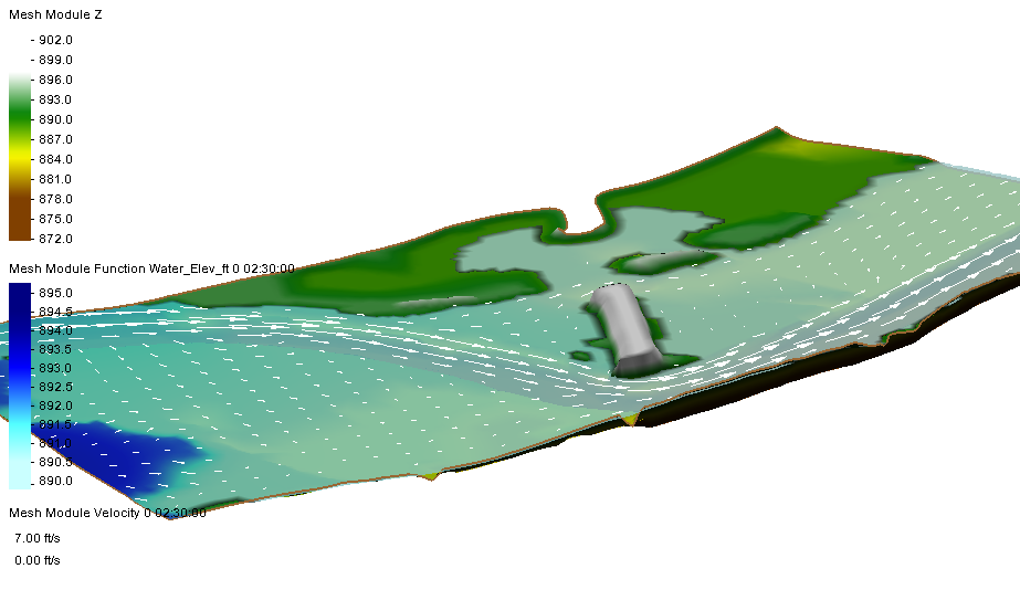
This option is available for all modules that allow displaying vectors. This includes the 2D mesh module, Cartesian grid module, quadtree module, and scatter set module.
There is also an option to specify an offset for the selected dataset. For example, you could set the offset to 1 or 2 to get the vectors slightly above the surface. The result would show the vectors mapped 1 or 2 feet above the ground elevation.
This addition to the vector display option can be used with any dataset in the same module. Therefore, any dataset in the mesh module can be used with a mesh, any dataset in the scatter module can be used with a scatter set, etc.
Try out using the new "Relative to dataset" vector display option in the SMS 13.1 beta today!