Solution for Overlapping Points in MODFLOW
By aquaveo on October 24, 2023When using the Groundwater Modeling System (GMS), it is important to understand how cells work in MODFLOW models, especially with conceptual models. Conceptual MODFLOW models are defined using feature objects such as points, arcs, and polygons on a grid. GMS processes each feature object separately, and occasionally there may be more than one feature object in a cell. MODFLOW is able to handle more than one boundary condition in a cell simultaneously, however, there are some things you should note.
The use of coordinates is essential to GMS as a whole, but not to MODFLOW. GMS uses coordinates to keep track of the exact location of feature objects relative to each other, as well as relative to the grid and other model data. Because the cell is the smallest unit of measurement in MODFLOW models, it only cares about the contents of the cell and not the specific location within it. All feature objects within the cell are mapped to the cell center and used for the cell calculations simultaneously.
When importing MODFLOW data that wasn't created in GMS, there are no coordinates tied to that data, so GMS uses the cell center as a reference and places all points there. This poses a problem as GMS requires that all points are assigned to unique coordinates, so GMS will generate an error message if any two or more points share an x, y, and z location. The way to fix this is pretty straightforward, although it can become tedious depending on the number of points on your grid. To solve this problem, follow these steps:
- Open the Attribute Table dialog by double-clicking on a point in the Graphics Window.
- Make sure the Feature type is set to "Points", and the Show dropdown is set to "All".
- Check the box next to Show coordinates.
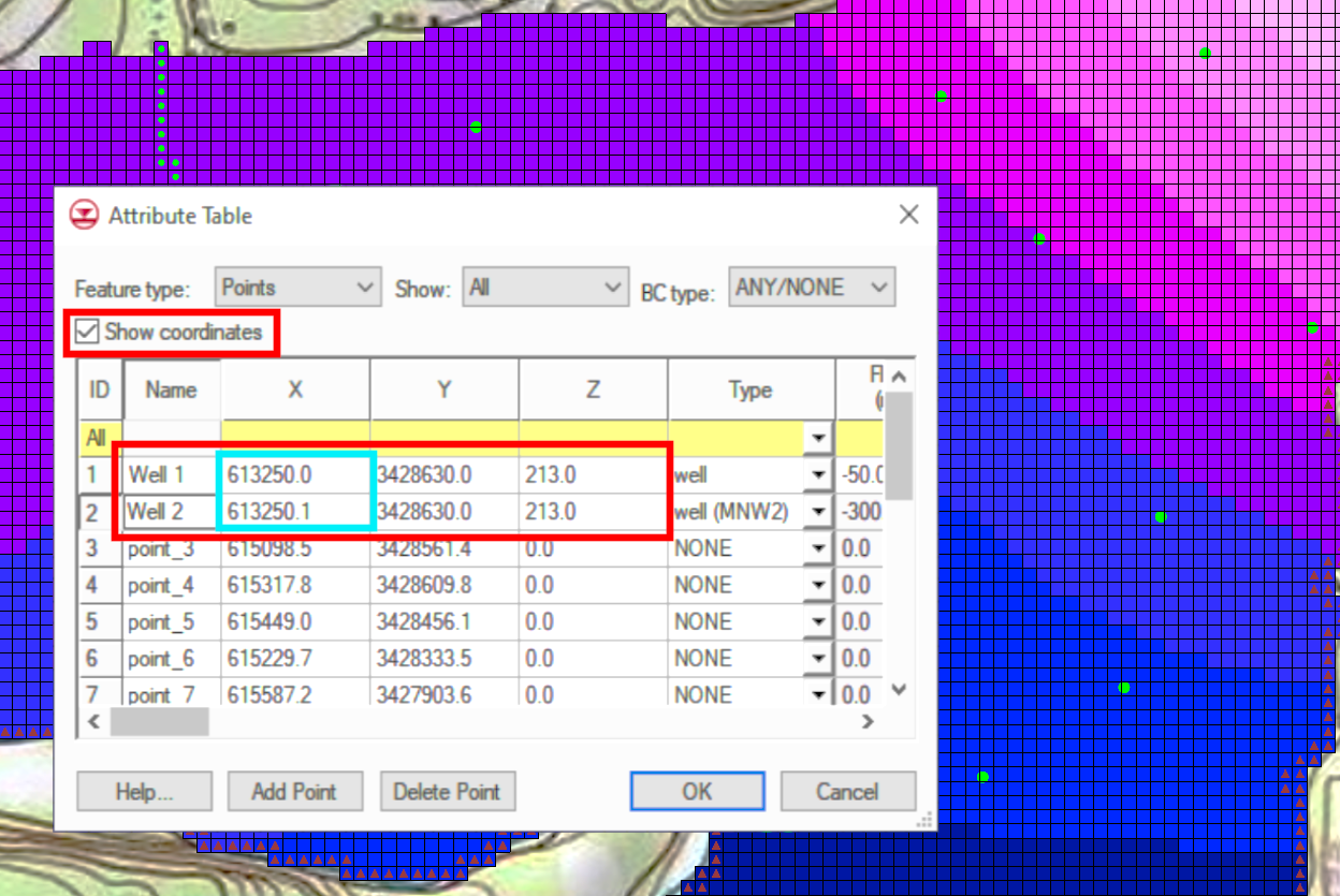
Now you can identify which points share the same coordinates and make the necessary changes. GMS only cares if more than one point has exactly the same coordinates in the x, y, and z directions. Offsetting a point even slightly in one of the three directions is enough for GMS to no longer have a problem, and the calculations will come out the exact same as long as the point remains within the original cell.
Head over to GMS and use these tips to make sure your MODFLOW simulation runs smoothly!