GMS

Setting Up a Cross Section Animation in GMS

By aquaveo on March 28, 2023

Have you ever wanted a way to better visualize cross sections in your project? The Animation Wizard in the Ground-water Modeling System (GMS) can help you do just that. Any project involving a 3D mesh or 3D grid can utilize the cross section animation feature.

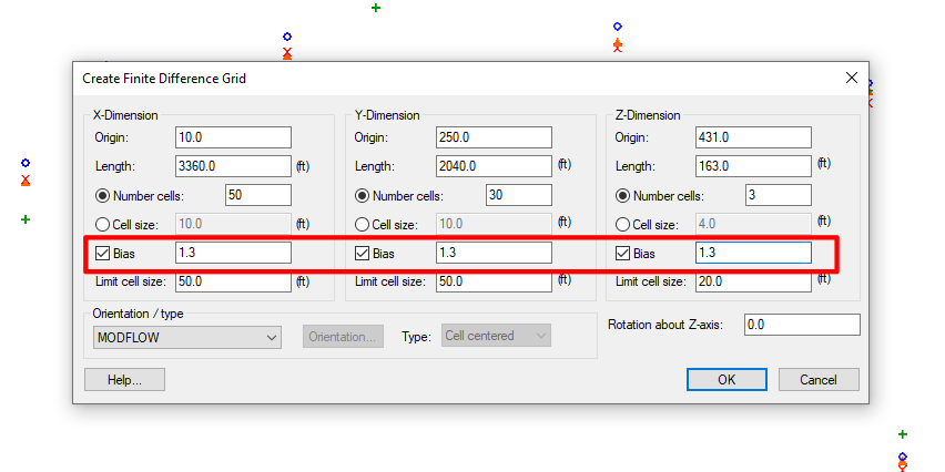
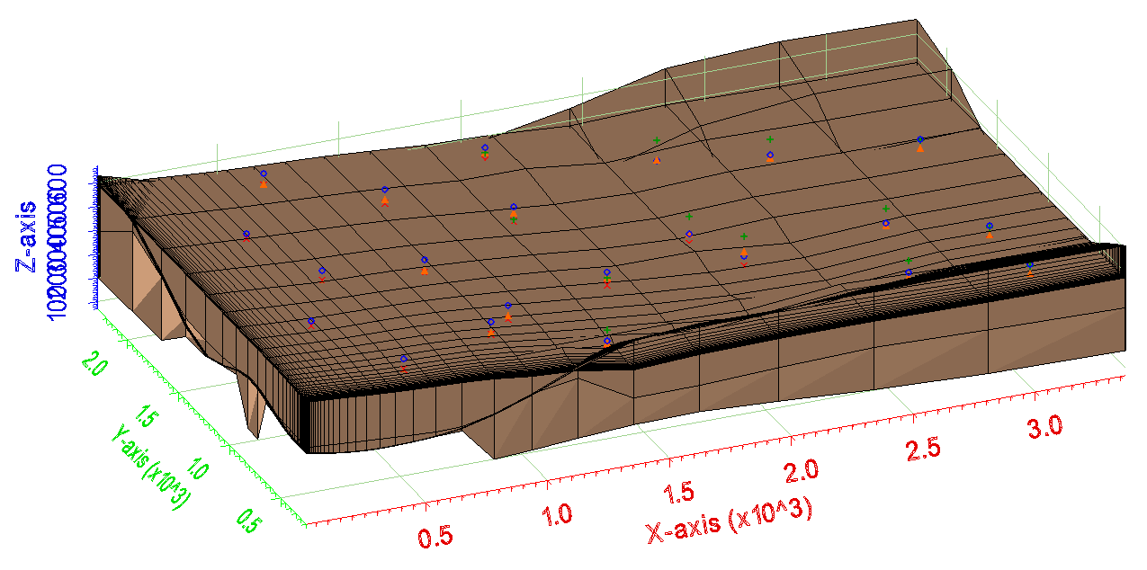
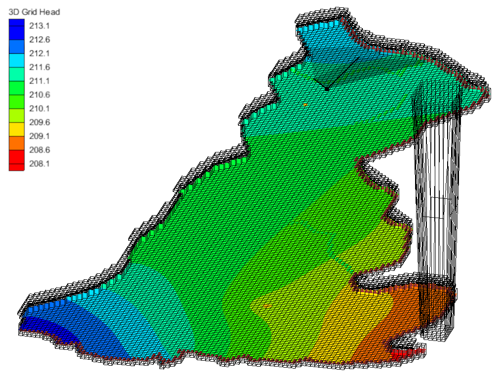
To build your initial cross section, you’ll need to start with a 3D mesh or grid as a foundation. After your foundation is set, build the cross section. Keep in mind that the Animation Wizard will create the animation through what is currently visible in the Graphics Window, so it is a good idea to get the display settings where you want them before starting the animation process.

Go to the Display menu and scroll down to the bottom to find the Animate option. Before initiating the animation, make sure that the cross section is active in the Graphics Window. Note that although the cross section needs to be active to create the animation, it doesn’t need to be turned on if you don’t want the static cross section from the project to be visible.

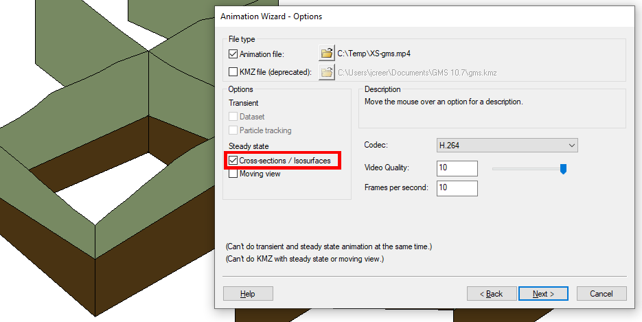
Example of the setting up a cross section animation in GMS

In the Animation Wizard dialog, turn on Cross-sections/Isosurfaces under Steady State. This is the option that animates the cross sections. You can change the speed of the animation by altering the number of frames per second, which is on the first page of the Animation Wizard, and the number of frames, which is on the second page. The lower the number of frames per second, the longer the animation will spend on each cross section, and vice versa.

The second page of the Animation Wizard is where you can specify the plane over which the cross sections will be animated. You can animate over the X, Y, or Z-axis, or any combination of the three. You can also alter more of the display options for the animation under the Cross Section Option button on this page.

After clicking Finish, the Animation Wizard will automatically export the cross section animation as an MP4 file, and you can open the MP4 file to view the finished product.

Even more settings and options are available that were not covered in this post, explore what cross section animations can do for your GMS project today!

Blog tags:

GMS

Using Bias When Creating a 3D Grid

By aquaveo on March 7, 2023

Sometimes when creating a 3D grid in the Ground-water Modeling System (GMS) you may want to include a bias in the grid for your project. Using a bias parameter will refine part of the grid along a particular axis. Here are some important things to know when implementing a bias into the grid.

All of the data fields necessary for this function will be in the Create Finite Difference Grid dialog window, which appears when a new grid is created. It is here that you can customize the X, Y, and Z-Dimensions to include your bias. The starting point for the bias is determined by the cell number designated in the Origin field of each dimension, and the bias will run along the axis in the positive direction. You can input a different value for the bias in each of the dimensions.

Example of the Create Finite Difference Grid dialog showing the bias option

For a value greater than one in the bias field, each cell will be a percentage larger than the one previous. For example, a bias of 1.2 will mean that each cell following the origin is 20 percent larger than the one previous. These cells will grow in the positive direction along the axis. To make each cell following the origin smaller than the one previous rather than larger, make the bias less than one. For example, a bias of 0.8 will mean that each cell will be 80 percent of the size of the previous cell.

The length field in each of the dimensions determines the total length of the dimension. All of the cells on that axis will fit inside that measurement. After specifying a length, there are two options for how GMS will calculate the size of the cells including the bias. First is by the number of cells in each axis. The grid creator will calculate how big each of the cells must be in order to fit that number into the specified length.

The second option for determining cell size is to input a value for the dimension of the starting cell. For example, setting the cell size to 10 feet will tell the grid creator that the origin cell should be 10 feet, and each cell following should be a percentage larger than the origin cell until the entire length of the axis is filled. This can be refined even farther by specifying a cell size limit, keeping a cell from growing larger than a specified size. Because of this, the cell size limit should be set to a number larger than the base cell size.

With GMS, there are many ways to customize a 3D grid. Give the grid bias function in GMS a try today!

Blog tags:

GMS

Working with Inactive Cells in MODFLOW 6

By aquaveo on February 14, 2023

When working with a MODFLOW 6 model in the Groundwater Modeling System (GMS) it can be important to mark specific cells inside a project as inactive to keep it out of the computational domain. Using inactive cells can speed up the performance and accuracy of your model. Incorrectly designating cells as inactive or active can cause inaccuracies in your model or keep it from converging. Here is some guidance for working with inactive cells that will help create a better MODFLOW 6 model.

Modflow 6 model with inaccurate z values

When choosing which cells to mark as inactive in GMS, it is helpful to know how to find information about the cells in the first place, as well as what information MODFLOW 6 is using to calculate the X, Y, Z, and S values of that cell. The display above the graphics window that shows the values of the selected cell is using the cell center for its calculated values. If the inactive cells have a low elevation that is inaccurate for the model, it will drag the Z value for the active cells on the edge down to meet the inactive cell. This happens because the outside active cell has nodes in the Z value that still need something to attach to as there cannot be gaps between the nodes. This will distort the cells in unintended ways and create errors in the model.

MODFLOW 6 uses IBOUND to determine which cells to mark as active and which to mark as inactive. Marking a cell with an IBOUND value of zero will make it inactive.

There are a few ways to inactivate cells in a MODFLOW 6 model. The first is to create a polygon that will separate the active and inactive cells. Select the polygon that contains the cells that are to remain active. Go to the Feature Objects menu and select Activate Cells in Coverage(s). This will automatically make any cells that aren’t selective inactive.

The second way is to select a group of cells with the cell selection tool. Then go to the MODFLOW menu | Advanced | Cell Properties… and change the IBOUND dropdown menu to inactive. This will inactivate only the cells that have been selected in the graphics window.

The cells can also be set as inactive by editing the IBOUND Array directly.The IBOUND dialog can be found by clicking on Global Options under the MODFLOW menu. There is an IBOUND button in this dialog window where the IJK coordinates can be set to zero manually.

Making use of inactive cells can improve you MODFLOW 6 model. Try out MODFLOW 6 in GMS today!

Blog tags:

GMS

Converting Between 2D and 3D Unstructured Grids

By aquaveo on January 17, 2023

Many projects in the Groundwater Modeling System (GMS) start with an unstructured grid (UGrid). GMS supports both 2D and 3D UGrids. The type of UGrid you will need to use will depend on which numeric model you are using for your project. For this reason you may need to change a 2D UGrid to a 3D UGrid or vice versa. This blog post is going to review some of the tools for converting between 2D and 3D UGrids.

Typically, models like MODFLOW-USG or MODFLOW 6 will require a 3D UGrid. If you only have 2D UGrid data, this may require taking a 2D UGrid and converting it to be a 3D UGrid. Likewise, you may need to convert a 3D UGrid to be a 2D UGrid. This is more often done to correct uses with the 3D UGrid, but also to be able to use the data from the 3D UGrid with other applications.

GMS provides two tools in the Toolbox for changing between 2D and 3D UGrids: the Extrude to 3D UGrid tool and the UGrid 2D from UGrid 3D tool. The Toolbox is accessible through the Toolbox macro and these two tools are located with the Unstructured Grids tools.

Example of the Unstructured Grid tools in GMS

The Extrude to 3D UGrid tool converts a 2D UGrid to a 3D UGrid. The tool will allow you to select a 2D UGrid for extrusion, and then it lets you specify the number of layers and layer thickness for each of the new layers. This will extrude the 2D Ugrid to be a 3D UGrid with the specified number of layers that are at a uniform thickness. If you need layers to be at different thicknesses, you will need to edit the 3D UGrid using other tools in GMS.

The UGrid 2D from UGrid 3D tool will collapse a 3D UGrid to be a 2D UGrid. The tool allows you to select a 3D UGrid then select if the 2D UGrid should be created from the top or bottom of the 3D UGrid layers.

The unstructured grid tools in GMS allow you to have more options with how you work with UGrids and grid data for your groundwater projects. Try out the unstructured grid tools in GMS today!

Blog tags:

GMS