Utilizing PEST Observations with MODFLOW 6
By aquaveo on September 12, 2023MODFLOW 6 comes with an observation utility (OBS) in the Ground-water Modeling System (GMS). This allows you to calculate values like water levels, drawdown, and flow for specific locations throughout the simulation. This utility employs programs from PEST, which makes it similar to the observation feature available in GMS for MODFLOW-USG.
PEST was developed to be used in conjunction with complex environmental models. PEST is an inverse model that uses set parameters to launch the model multiple times until the output matches the observed values, eliminating the need for manual calibration of a MODFLOW simulation.
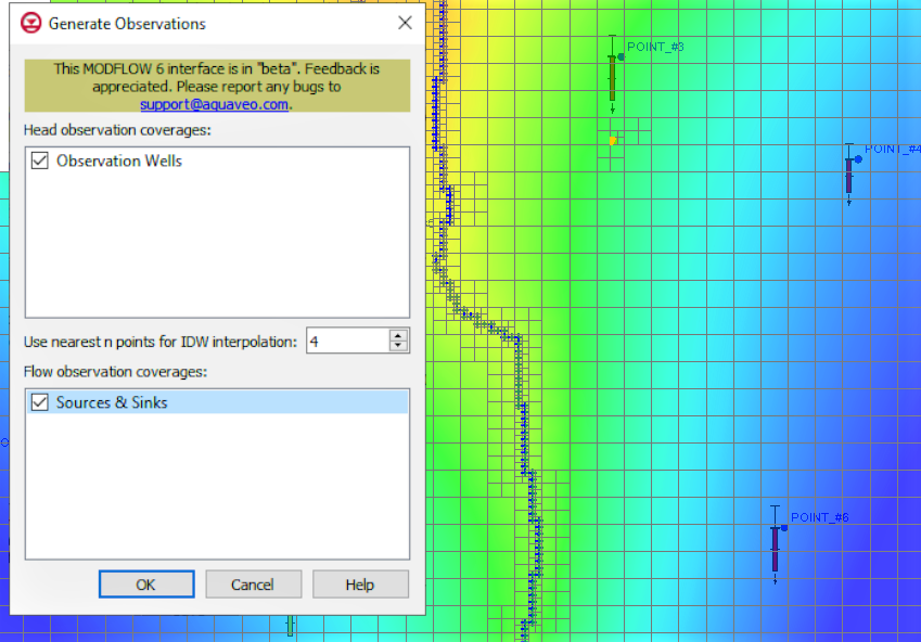
The way PEST Observations are added to MODFLOW 6 is different from how they are added to other versions of MODFLOW in GMS. With standard MODFLOW, observations are added to the simulation through the MODFLOW | Observations menu option. PEST observations are added to a MODFLOW 6 simulation by right-clicking on the simulation in the Project Explorer and selecting New Package | PEST Observations. This is where the PEST input data is generated for the simulation. The Generate PEST Observation Data button is what allows you to assign coverages as the head and flow observation coverages.
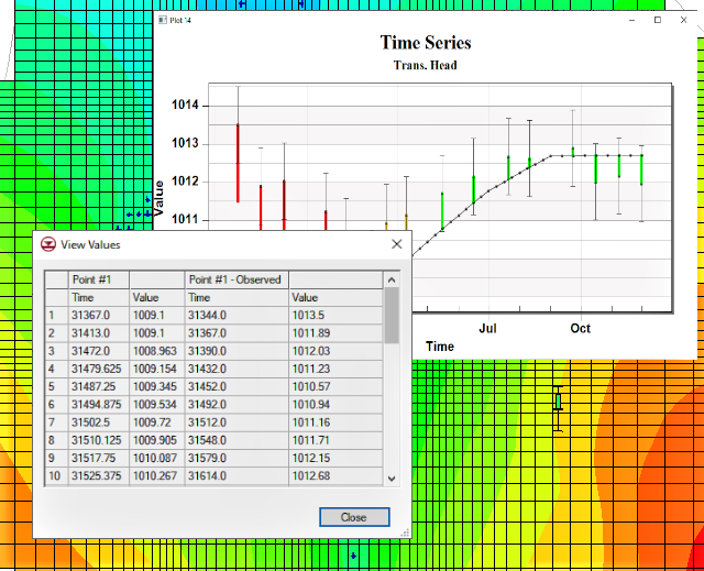
After running the simulation with PEST Observations, you can view the data using statistics tools, whisker plots, and observation plots. The statistics can be viewed in the form of a text file, which are found under the solution files folder in the Project Explorer. Running the MODFLOW 6 simulation with the PEST Observations package automatically generates new coverages with the observation arcs or points. The whisker and observation plots are accessed by making one of the new PEST observation coverages active, then selecting an observation point or arc in the Graphics Window.
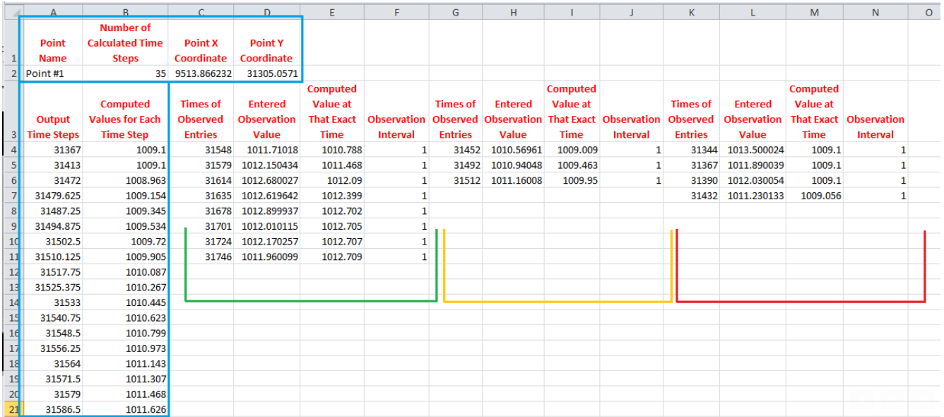
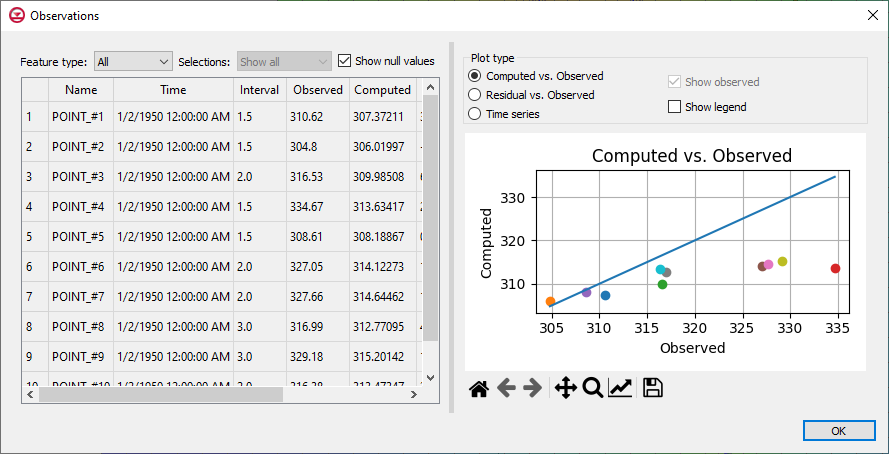
If you right-click on one of the PEST Observation coverages you can select Observations, which will bring up a dialog that contains a table with all the data from the observation arcs or points, as well as a plot that displays all of the points on a graph.
Adding PEST Observations to your MODFLOW 6 model can be incredibly useful, so head over to GMS and see how it can enhance your project today!