GMS

Announcing GMS 10.8 Beta!

By aquaveo on December 5, 2023

We are pleased to announce the release of GMS 10.8 in beta! There are many updates and additions that have been made in the newest version of GMS and this blog post will explore just a few of the new tools and functionalities.

HydroGeoSphere

HydroGeoSphere is a model brand new to GMS, which will be available to you in GMS 10.8 beta. The HydroGeoSphere model was developed by Aquanty to accurately replicate the intricate processes involved in the terrestrial part of the hydrological cycle using a three-dimensional control-volume finite element simulator.

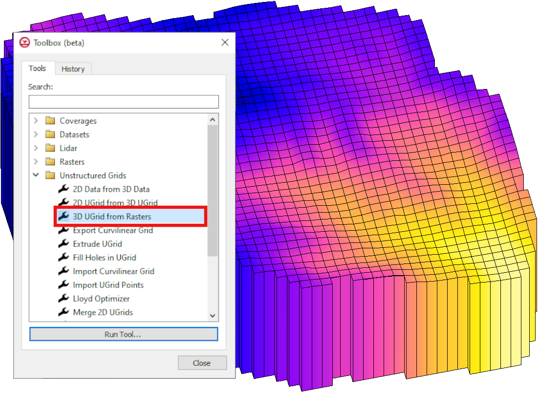
3D UGrid from Rasters

The 3D UGrid from Rasters tool is new to the GMS toolbox. This tool is found under the Unstructured Grids folder in the toolbox, and can be used to generate a 3D UGrid using multiple rasters and a 2D UGrid. It creates layers between the rasters using the 2D UGrid and the horizons approach. When this tool is used, the resulting 3D UGrid has no vertical sub-discretization of the layers, and the horizontal discretization of all the layers is the same. More information about this tool can be found on this page of our wiki.

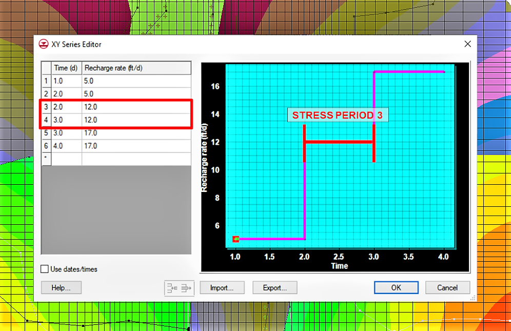
MODFLOW-USG Transport

MODFLOW USG Transport in GMS has new support for seepage elevation and concentration in the Recharge (RCH) package. The Evapotranspiration (EVT) package now supports ETFACTOR.

Color Ramp

The way the color ramp in the contour display options works has been updated, and many new color options have been added to GMS 10.8. The way the color ramp works has been changed to more closely resemble the changes that have already been made in SMS and WMS. If you want a more detailed explanation of how to use this version of the color ramp, you can check out this blog post. The blog post covers the color ramp for SMS, but the functionality is basically identical between SMS and GMS.

There are a lot of new things to try in GMS 10.8 beta, so download it from our website and check it out today!

Blog tags:

GMS

Utilizing the Transient Step Function Method

By aquaveo on November 14, 2023

The Groundwater Modeling System (GMS) provides tools for working with transient MODFLOW simulations. When working with transient dataM in a MODFLOW model, it is important to understand stress periods and how GMS calculates their values. There are two different methods you can use to define the values for a stress period: the continuous time series method, and the step function method. This blog post will cover how to input the data for a stress period in the XY Series dialog so that GMS will calculate their values correctly.

Transient MODFLOW simulations use time intervals called stress periods to define the values of transient stresses such as pumping rates, and river stages. The values for stress periods are entered in the XY Series dialog, which is opened from the Attribute Table dialog. For a continuous time series, you need to enter only one data point per time step. When you enter only one value per time step, GMS assumes that the value continues to increase through the stress period, creating a straight line connecting the two points for a smooth transition. But because GMS needs a constant value for each stress period, it will take an average of the starting values of that particular stress period and the starting value of the following stress period.

The step function method tells GMS that there is only one value for each stress period, rather than a continuously increasing value. To input data in the XY Series dialog so that GMS knows that there is only one constant value through the entire stress period, you’ll need to enter both a start value and an end value. The figure below shows an example of the format to use.

As you can see in the above figure, you need the end value of a stress period to match the start value of the following stress period. This creates "steps" in the data, telling GMS to read a constant value through the entire stress period, rather than having a gradual increase from beginning to end.

Head over to GMS and try creating a step function for your transient MODFLOW model today!

Blog tags:

GMS

Solution for Overlapping Points in MODFLOW

By aquaveo on October 24, 2023

When using the Groundwater Modeling System (GMS), it is important to understand how cells work in MODFLOW models, especially with conceptual models. Conceptual MODFLOW models are defined using feature objects such as points, arcs, and polygons on a grid. GMS processes each feature object separately, and occasionally there may be more than one feature object in a cell. MODFLOW is able to handle more than one boundary condition in a cell simultaneously, however, there are some things you should note.

The use of coordinates is essential to GMS as a whole, but not to MODFLOW. GMS uses coordinates to keep track of the exact location of feature objects relative to each other, as well as relative to the grid and other model data. Because the cell is the smallest unit of measurement in MODFLOW models, it only cares about the contents of the cell and not the specific location within it. All feature objects within the cell are mapped to the cell center and used for the cell calculations simultaneously.

When importing MODFLOW data that wasn't created in GMS, there are no coordinates tied to that data, so GMS uses the cell center as a reference and places all points there. This poses a problem as GMS requires that all points are assigned to unique coordinates, so GMS will generate an error message if any two or more points share an x, y, and z location. The way to fix this is pretty straightforward, although it can become tedious depending on the number of points on your grid. To solve this problem, follow these steps:

Open the Attribute Table dialog by double-clicking on a point in the Graphics Window.
Make sure the Feature type is set to "Points", and the Show dropdown is set to "All".
Check the box next to Show coordinates.

Now you can identify which points share the same coordinates and make the necessary changes. GMS only cares if more than one point has exactly the same coordinates in the x, y, and z directions. Offsetting a point even slightly in one of the three directions is enough for GMS to no longer have a problem, and the calculations will come out the exact same as long as the point remains within the original cell.

Head over to GMS and use these tips to make sure your MODFLOW simulation runs smoothly!

Blog tags:

GMS

How to Refine an Unstructured Grid

By aquaveo on October 3, 2023

When working with a multi-layer unstructured grid (UGrid) in the Ground-water Modeling System (GMS), your project may require different levels of refinement in each layer to introduce complexity to the stratigraphy. GMS currently offers a limited number of ways to achieve this in a 3D UGrid module. Mapping coverage directly to a 3D grid simplifies vertical refinement considerably, but it results in all layers being of uniform size. This blog post will cover the most straightforward way to create a complex stratigraphy, as well as some things that may be useful to know about how refining grids works and what the limitations are.

The type of grid that will often get you the closest to where you want to be is a Quadtree grid. These are the steps you’ll want to follow:

Using the Refine command to refine a quadtree

Use the TINs/Horizons to UGrid approach to generate a grid that incorporates the desired pinchouts and ensures an appropriate level of refinement for the least refined layer.
Right-click on the Quadtree UGrid in the Project Explorer and scroll to the bottom of the UGrid Properties dialog window.
Make sure the Constraint dropdown is set to "None". If the constraint is set to "3D", you will not be able to refine the UGrid cells.
In the toolbar above the Graphics Window, check the box for Single Layer to isolate a layer of the grid for refinement. Highlight the cells you wish to refine using the Select Cells tool.
Right-click on the selected cells and choose Refine.

The newly generated UGrid maintains the original level of refinement on all layers except for the one where you just refined some of the cells. You can repeat this process as many times as needed to achieve the desired level of refinement.

Currently, there is no automated process for this kind of complex refinement, so while it is possible to use this process on a larger project, it may not be practical. If you have a limited number of areas to work on, this workflow lets you produce a grid that features your desired TIN pinchouts, with varying levels of refinement for different layers. It is also not possible to un-refine a grid, so you’ll always need to start with the least refined layer and work your way to the most refined.

Head over to GMS and try this method to refine your 3D grid today!

Blog tags:

GMS