GMS

Changes to Aquaveo Registration

By aquaveo on March 10, 2021

Aquaveo has been updating its registration process to make using our products easier and more secure. The change affects newer versions of our products, specifically GMS 10.5, SMS 13.1, and AHGW 3.5. Going forward, it will be added to all of our products, including WMS.

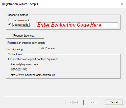
The new registration uses new codes: Local and Flex codes.

Local password: will support virtual machines and remote desktop, but is only good for one machine and cannot be moved from one computer to another.
Flex password: acts like a network lock where the license is hosted on your computer and can be used over remote desktop or on a virtual machine. When you want to move the license to another computer, you simply check the license back in and check it out on another machine. There is no hardware to deal with.

By default the software is set to use the newer registration process with newer versions of the software. Local and Flex codes are not compatible with older versions of our software.

In many cases you won't notice a difference with the change to licensing. However, if you encounter an error with your registration or want to use the older licensing process, you can switch back to using the old registration.

Open the newly installed software.
Choose to run it in Community Edition, if the "no license found" dialog appears.
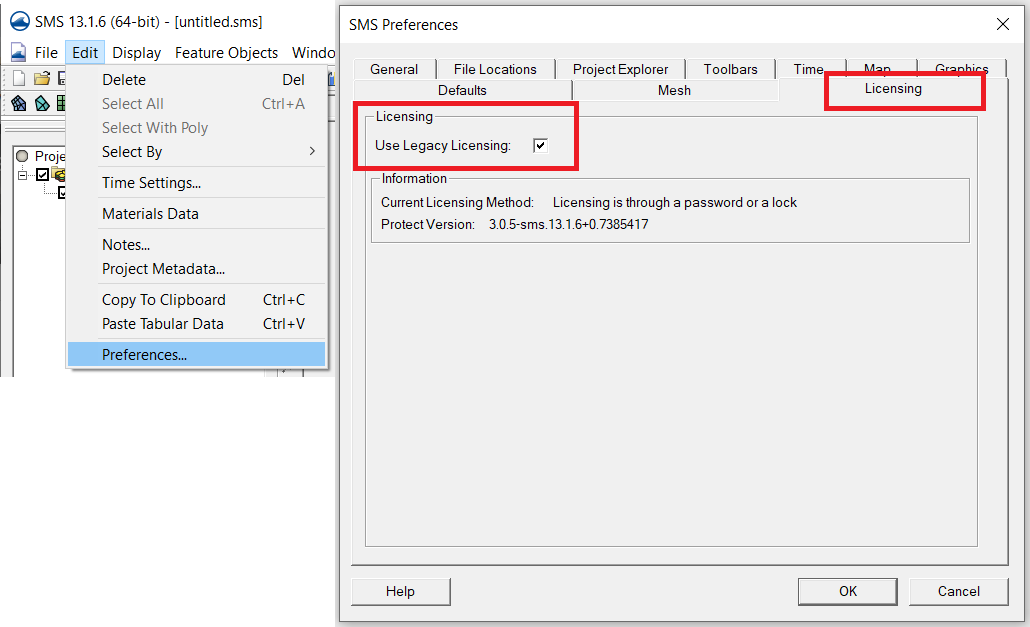
Once the software is open, go to Edit | Preferences.
Click on the Licensing tab.
Check on the box for "Use Legacy Licensing".
Click OK and restart the software.
Then register the software as you have before.

Currently, we plan on supporting hardware locks and the legacy registration version for at least the next two years. If you want to try out the new registration system, contact our licensing team at licensing@aquaveo.com.

Blog tags:

GMS

SMS

WMS

AHGW

Plotting Conductance for the DRN Package

By aquaveo on February 24, 2021

Are you looking for a way to contour the conductance of drainage areas in your groundwater model? If you have a large regional model containing areas with a dense drainage network (ditches, tile drainage, etc.), you can scale up this to represent a diffused drainage system. When doing this, there are not only single ditches simulated with the drain (DRN) package, but whole areas. Using GMS, you can create a contour of these drainage areas.

To create this contour, use the following workflow:

Go to MODFLOW | Optional Packages | DRN to open the Drain (DRN) Package dialog.
Make sure IJK is selected on the bottom in order to have the drains at their XYZ locations.
Click the top left blank grey box to select all or select and drag to select all the data points.
Copy the data and paste in a word processor such as Notepad++ and save the file.
Back in GMS, select Open File and select the new text file. The text wizard should open up and already have delimited the file, but double check to make sure all the values are correct.
Click Next then change the GMS data type to 3D Scatter points.
If your file included elevations, you can make sure those are not mapped into your project by changing the dataset above to "Not Mapped".
Otherwise, make sure your IJK cell values are matched up with their respective XYZ values and your conductance is set as the "Dataset".
You may have to select the projection for this dataset in order for it to line up with your current project.
You can then go to Display Options, select 3D scatter points on the left sidebar, and then turn on Contours if it has not already been turned on. You can check the contour options to see if the setup and coloring is to your liking.

Completing this workflow should cover all the drain points within the MODFLOW project. Try out contouring drainage areas in GMS today!

Blog tags:

GMS

Troubleshooting Importing Boreholes in GMS

By aquaveo on February 3, 2021

Have you encountered issues when importing borehole data into GMS? The majority of the time, there are no issues when borehole data is imported into GMS, but occasionally something becomes misaligned. This article will attempt to address some of the common issues that occur when importing borehole data.

The most common issue happens when the borehole data file is formatted incorrectly for GMS. Often this can be fixed when importing the borehole through the File Import Wizard. Selecting the correct options in the File Import Wizard can resolve many issues. However, in some cases the borehole data will need to be reformatted using a spreadsheet program or text editor. If this is the case, follow the recommended borehole file format.

Another issue occurs when importing borehole data happens when the coordinate system for the borehole data does not match the coordinate system for the GMS project. When this happens, all of the boreholes will be unaligned with the project data or it may happen that all of the boreholes will be stacked on top of each other. This latter case typically occurs when the borehole coordinates are in latitude and longitude, but the GMS project is using a projected coordinate system, which would use linear units such as feet or meters.

To fix this issue, the correct projection needs to be set for the boreholes. This is done by doing the following:

In the Project Explorer, right-click on the imported boreholes and select the Projection command.
In the Object Projection dialog, set the projection to match the project projection.

With the correct projection set, the boreholes should line up with the project data.

Additional adjustments to boreholes can be made using the Borehole Editor. This is accessed by right-clicking on the borehole and selecting the Properties command. This method is best when only a few boreholes are imported incorrectly. If several or all boreholes were imported incorrectly, it is recommended to review the borehole data and fix any issues before importing into GMS.

For further troubleshooting with importing borehole data, contact our technical support team at support@aquaveo.com. Try out using boreholes in GMS today!

Blog tags:

GMS

Using Evaluation Versions of GMS, SMS, and WMS

By aquaveo on January 27, 2021

Are you wanting to try out GMS, SMS, or WMS, but aren’t quite ready to commit to purchasing a license? Or maybe you have a license, but your maintenance has lapsed and you’d like to check out the new features in a beta version before updating your maintenance?

Aquaveo permits using an evaluation license for its products to permit you to try out our software to see if it will meet your needs. Evaluation licenses are temporary license codes that let you use all the functionality of our software for two weeks.

To receive an evaluation license code, do the following:

Download the software you want to evaluate from our downloads page.
After downloading and installing the software, use the Request License button in the Registration Wizard to go to the Software Evaluation Request page on our website.
Fill out the request form and an evaluation license code will be sent to you.
Register the software using the evaluation license code sent to you.

After registering the software with the evaluation code you will be able to use all of the software functionality to determine if the software will meet your water modeling needs. Note that evaluation licenses are only for evaluation purposes and are not intended for creating finished models. It should also be noted that certain third party models, such as TUFLOW or Hydro AS-2D, will still require a separate license in order to fully evaluate them.

After the two week trial period, the license will expire and you will no longer be able to use the software until a paid license code is entered. You are only permitted one evaluation license per product per version.

If you encounter problems with registering an evaluation license, contact our support team at support@aquaveo.com. If you started an evaluation license and were unable to use the license during the evaluation period, contact our licensing team at licensing@aquaveo.com.

Blog tags:

GMS

SMS

WMS