How and When to Use Depression Points in WMS
By aquaveo on September 19, 2018Have you ever wondered what depression points are used for? Should you be including them in your watershed delineation? Depression points can greatly help to improve the accuracy of your model when used correctly.
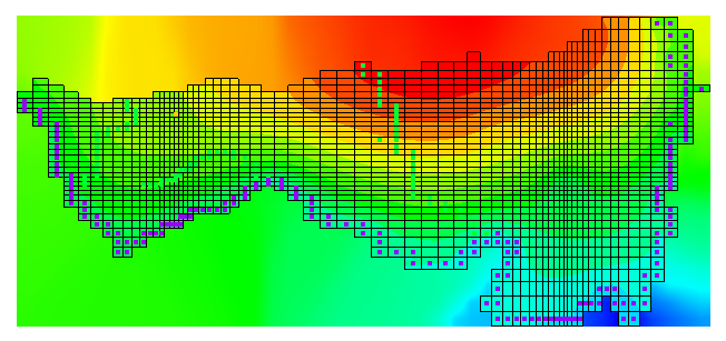
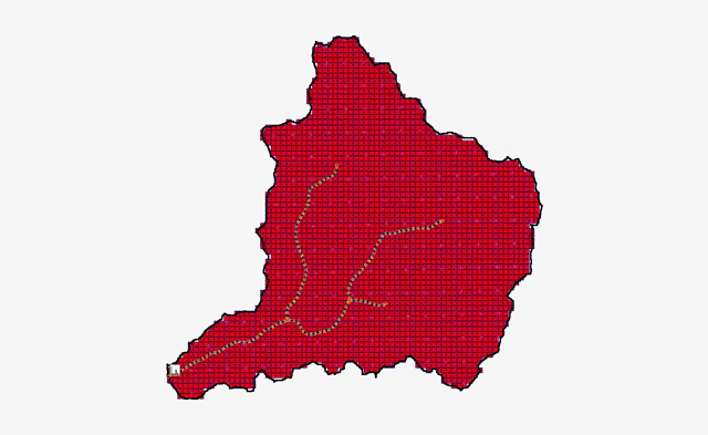
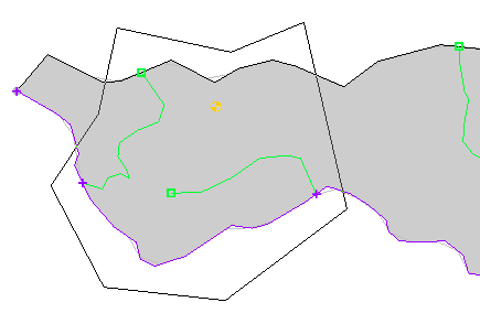
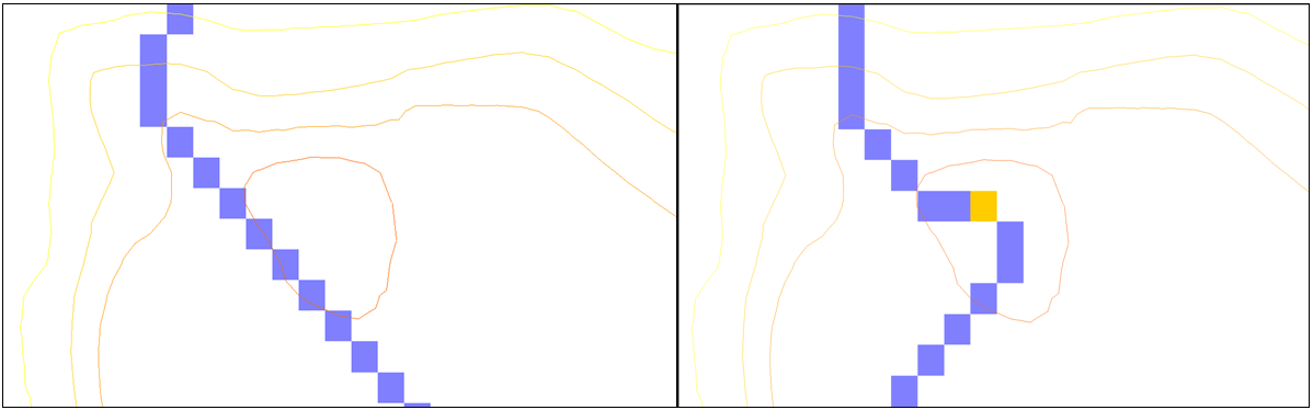
A depression point is significantly lower than its surrounding elevation, causing a change in flow accumulation and direction. An example of a depression area would be a watershed that contains a mine. TOPAZ is a public domain program that is used in computing flow directions and accumulations for use in basin delineation with DEMs. TOPAZ assumes that all depression points it encounters in its calculations are due to a lack of resolution, and therefore “fills” the depression point in increments until a flow path can be established straight across the low point. In order to view how a natural depression point would affect flow direction and accumulation, it is necessary to define the specified areas as depression points. This causes TOPAZ to read the cell as a NODATA cell, making TOPAZ think it is a DEM boundary instead of raising the elevation in the depression. Comparing a before and after of marking a depression point shows how the flow path is affected by depression points as displayed below.
It is appropriate to use a depression point where a natural depression occurs in the horizon. Typically you would only define depression points for larger areas where the flow path will be significantly affected by the area. It is not always necessary to define a depression point however. You want to use it when you receive straight lines for delineation boundaries for instance. This would most likely be caused by undefined depression points.
Some errors can occur however when defining depression points incorrectly.
- Sometimes users will mark the bottom elevation that is actually up higher to the side of the depression point and is not exactly the center deepest point. This issue can be avoided by using the Set contour min/max tool in the Terrain Module to correctly identify the absolute bottom elevation. This DEM point is the one which should be marked as a depression point.
- Another incorrect use of depression points would be to use them to outline where a stream bed is. A stream bed can be identified by using stream arcs in WMS.
Now that we’ve established when and when not to use depression points, you might be wondering how to create depression points in WMS. To create depression points in WMS:
- Turn on the Terrain Data Module.
- Use the Select DEM points tool to select the cell containing the lowest DEM elevation. If working with an area that has a large natural depression, simply hold down the Shift key to select all of the cells with low elevation at once.
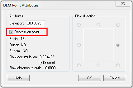
- Select DEM | Point Attributes to bring up the DEM Point Attributes dialog.
- Turn on Depression point to mark the cell as a depression point.
Now that the depression points are set, you can run TOPAZ to view the new flow paths. TOPAZ will recognize the new depression, and the detention basin calculator can be used to create a stage-storage curve.
Try adding depression points in your WMS model today!