How to Calculate Riprap Using the Hydraulic Toolbox
By aquaveo on November 28, 2018
Are you needing to determine the size of stones needed for riprap? Having stones that are too small will reduce the effectiveness of the riprap which could be disastrous. On the other side, having stones that are too large could cause unnecessary expense.
After defining drainage data in WMS, it is possible to calculate the riprap needed for your model using the FHWA Hydraulic Toolbox. To do this:
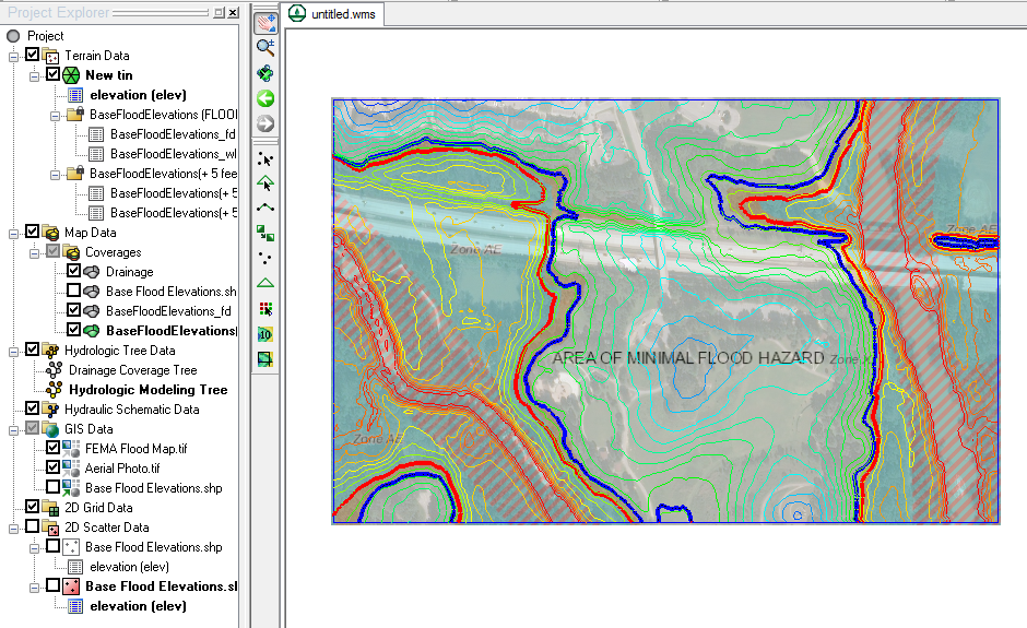
- Define your drainage data in WMS.
- Assign each basin attribute to an analysis method by double-clicking on the feature, and then selecting Edit Attributes…. This will give you the opportunity to link your drainage data to the Hydraulic Toolbox.
- Click on the Hydraulic Toolbox
 macro in WMS to bring up the Hydraulic Toolbox.
 - You can calculate riprap using one of two methods:
- Channel Lining Design Analysis Tool. Keep in mind when using this tool that a filter material must be separately designed.
- Riprap Analysis Tool. This tool will calculate the filter material along with riprap size.
Once in the Hydraulic Toolbox, locate the name of the analysis method chosen and double-click to open the analysis dialog for the chosen parameter and method. You will notice that all of the data you input into WMS is now filled in the analysis tool. After you specify blank parameters, the tool will calculate and display the results at the bottom of the screen under “Minimum Riprap Thickness”.
Using the Hydraulic Toolbox to calculate riprap can help your project move forward. The toolbox also contains many other features worth exploring. Try using the Hydraulic Toolbox today!


 ]
]