Using STL Files in SMS
By aquaveo on June 26, 2019Starting in SMS 13.0, SMS can now make use of STL files.
STL files use tessellation, the process of mimicking a surface by assigning surface coordinates to a repeated pattern of polygons. In the case of STL files, triangles are used to make a 3D mesh that can effectively be rendered into any shape needed including landscapes.
STL files are typically used for 3D printing. They also can be used for the modeling landscapes. There are several methods for creating these files. This post will not attempt to cover the specifics of those methods as other places cover how do this.
Uploading and Using STL Files
In SMS, STL files are used to model terrain. Once you have created an STL file, importing it by using the File | Open command or dragging-and-dropping the file into SMS.
When uploaded, the file is automatically transformed into a Ugrid and adjusted for the associated z values. This UGrid can then be used for all the normal uses of such in SMS.
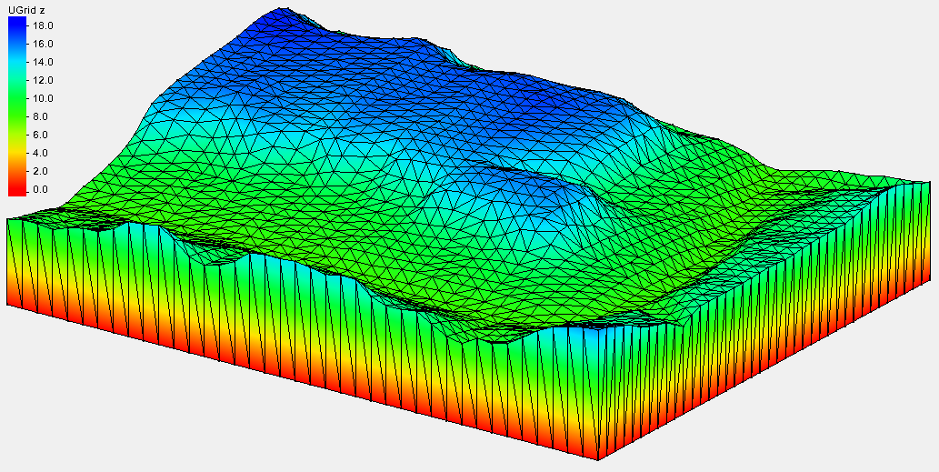
It is important to mention that the z values may or may not be representative of the elevation depending on the source of the STL file used. Fortunately, there is a way to handle such cases in SMS. After import, the Ugrid can be converted into a 2D scatter dataset. The scatter can then be interpolated to a mesh or modified with the data calculator. If desired, tim and dim files representing that data can then be created as usual.
Exporting STL Files
To create an STL file, you must have a UGrid with the corresponding elevation data attached. This UGrid must consist of only triangular elements.
Export the STL file by:
- Right-click on the UGrid and select the Export command.
- Then select a (*.stl) file type before saving the file.
There are two STL file type available for export. The binary option is often used since it requires less memory. The ASCII file is more user friendly if the file needs to be inspected. Both save data by recording the coordinates of the vertices associated with each triangle. If unaccompanied by other files, the Ugrid will also have to be manually associated with the correct projection after uploading.
We hope to add more functionality for STL files in the future. Try using STL files with your SMS projects today!