Tips for MODFLOW 6 in GMS 10.5 Beta
By aquaveo on June 10, 2020Have you had a chance to use MODFLOW 6 in the GMS 10.5 Beta? If you have, you may have noticed that MODFLOW 6 operates a little differently than other versions of MODFLOW. This is to allow for some additional tools and options.
When using MODFLOW 6 in GMS 10.5 Beta, here are a couple tricks to try out.
Having Multiple MODFLOW 6 Simulations in the Same Project
You can create multiple simulations in the same project by using the simulation workflow in GMS 10.5 beta. This is particularly useful when attempting to calibrate your project. The way this is done is by doing the following:
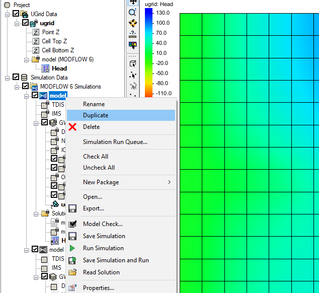
- Right-click on the simulation in the Project Explorer and select the Duplicate command. This will create a duplicate of the simulation that includes all the same parameters and uses the same grid.
- On the new simulation, change the parameter that needs to be calibrated, such as the head values or the pump values of the wells. It is generally best to only focus on one parameter change when calibrating the model.
- Run the new simulation and compare the results between the different simulations.
- Repeat this process with additional simulations to calibrate the model.
Running Multiple Simulations at the Same Time
After you have created multiple MODFLOW 6 simulations, you can run all of the simulations at once. This is done by doing the following:
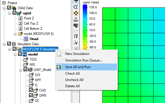
- Right-click on the simulation folder and select the Save All and Run command.
The Simulation Run Queue dialog will display all of the simulation model runs. While the simulations are running, the Simulation Run Queue can be moved aside or minimized to allow you to keep using GMS. The results can be loaded into the project for you to review when the simulations have finished.
Additional features for MODFLOW 6 are still being added to GMS and will appear in future versions of the software. For now, check out MODFLOW 6 in GMS 10.5 beta today!