SMS

Creating Reliable Arc Pairs for SRH-2D

By aquaveo on November 7, 2023

SRH-2D models in the Surface-water Modeling System (SMS) often use pairs of arcs to represent structures like culverts, weirs, bridges, and gates. For some projects, it matters for SRH-2D about how these arc pairs are drawn, and improperly drawn arcs can stand in the way between you and a successfully run model.

Arc pairs in SRH-2D models need to be drawn from left to right as if you are looking from upstream to downstream. This can get quite confusing, so here are a few tips for how to be able to tell which direction your arcs need to go by making use of display settings in the Display Options dialog.

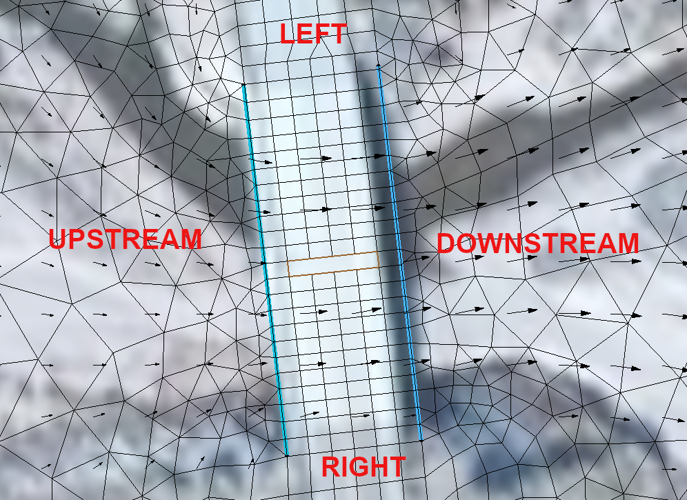
If you’re not sure which direction is upstream and which is downstream, select 2D Mesh from the list on the left of the Display Options dialog and turn on Vectors. This requires having a dataset associated with the mesh that contains vector values. The vectors will display the direction the water is flowing, which makes it easy to be able to tell where upstream is. Now, to draw the arcs in the correct direction, imagine you are standing upstream and looking downstream. Then start the arc on your left and end it on your right. Both arcs need to be drawn in the same direction.

What do you do if you’ve already drawn the arcs and then you try to run your simulation and it fails? If the failure is caused by misdrawn arcs, the error will read "Program stopped due to the following: Linked Pair nodestring direction is wrong; please reverse them". The fix is simple if you have only one pair of arcs on your mesh: select both arcs in the Graphics Window, right-click, and select Reverse Arc Direction.

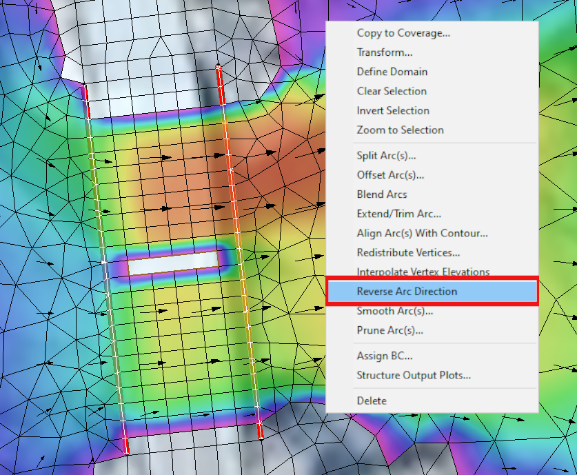
However, the existence of more than one arc pair can make solving this error a little more complicated. Rather than going around and either redrawing or reversing all the arcs, here's what you can do to pinpoint the problematic pair. First, open the Display Options dialog. On the Map tab check the box next to Annotations and click the Options button. In the Arc Annotation Options dialog, turn on Show arc direction arrow. Doing this will add arrows to the arc, pointing toward the end. This makes it easy to look at the arcs and see which ones are facing the wrong direction, at which point you can use the same steps as above to reverse the arc direction.

Head over to SMS and use this guide to help your SRH-2D model run more smoothly today!

Blog tags:

SMS

Using Mesh Auto-Backup

By aquaveo on October 31, 2023

Needing to save and reload older versions of your 2D mesh in the Surface-water Modeling System (SMS)? SMS 13.3 has a new set of tools that let you do just that. The Auto-Backup folder included in the Toolbox contains the Mesh Backup and the Mesh Reload tools. These tools let you save past versions of a 2D mesh while you are editing the mesh. If you discover a change to the mesh was undesirable, you can load a version of the mesh before the change was made.

SMS uses 2D meshes for a wide variety of models including, but not limited to, ADCIRC and SRH-2D, as well as generic models. Using the new Auto-Backup tools, you are free to make as many edits to the mesh as you need knowing you can recover the previous versions. This blog post reviews how the Auto-Backup tools work.

Mesh Backup Tool

The Mesh Backup tool creates a series of backups at specified intervals for a specified number of iterations. Both the interval and the number of backups are determined by the user in the tool’s dialog. The default values are a mesh backup every 20 seconds, 10 times. These values can be changed to whatever works best for your project, however, it is recommended that you limit the amount of backups to roughly 200 or less.

When you run the tool, a dialog labeled Turn on/off auto mesh backup will appear. This dialog means that the tool is on, and will run in the background while you work on your mesh. This dialog is intended to stay open while you work on your mesh. Clicking Cancel will turn off the tool. While the tool is running, SMS checks to see whether or not a change has been made to the mesh every time the specified time interval has elapsed, and then creates a backup copy.

The log portion of the Turn on/off auto mesh backup dialog keeps track of how many backups have been made for the mesh. It will also tell you if there was an interval where no changes were made to the mesh. In cases where no changes were detected, a backup copy of the mesh during that period will not be stored.

Mesh Reload Tool

The Mesh Reload tool is where you can access the mesh backups. Naturally, this means that you have to run the Mesh Backup tool before anything will be available to reload. The Mesh Reload tool dialog contains a dropdown menu with all the backup meshes labeled by timestamp. The dropdown menu will often not contain every single time stamp, because there will likely be some time stamps where no changes to the mesh have been made.

Using the Mesh Reload tool does not erase the current mesh, or backtrack any changes that you’ve made. It will simply add a copy of what the mesh looked like at that time stamp under the "Mesh Data" folder in the Project Explorer. Try out the new Auto-Backup tools in SMS 13.3 today!

Blog tags:

SMS

Using the Hydraulic Toolbox with SMS

By aquaveo on October 10, 2023

You may have already used the Hydraulic Toolbox to define a culvert for an SRH-2D model, but did you know its suite of calculators can assist you in many ways when creating a simulation in the Surface-water Modeling System (SMS)? The Hydraulic Toolbox is a software developed for the FHWA by Aquaveo, and there are many uses for the calculators, but today we’ll go over one example today to give you an idea of what you can do.

The Hydraulic Toolbox can assist you with calculations for other simulations, such as an SHR-2D urban hydraulics project in SMS. One of the main calculators that can be used for urban modeling with SRH-2D is the Curb and Gutter flow analysis.This calculator examines flow across storm drain inlets for various curb and gutter openings.

Example of the Hydraulic Toolbox with SMS

The Hydraulic Toolbox includes a macro that opens the Curb and Gutter Analysis calculator, or you can access it through the Calculators menu at the top of the window. This adds it to the Project Explorer under a “Project” folder. Once it has been added to the Project Explorer, double-click on the tool to open the calculator’s dialog. There are three main parts to the calculator: Gutter, Inlet, and a Parameters table. The Gutter section contains values for the gutter dimensions. This includes, but is not limited to, the gutter width, design flow, width of spread, etc.. The Inlet section is where factors defining the inlet location, inlet type, grate type, etc. are included. The Parameters table displays all the inlet data after it has been calculated by using the “Compute Inlet Data” button.

The Hydraulic Toolbox is separate from SMS, so as of SMS 13.3, data from the calculator will need to be entered manually into the relevant portions of SMS. The calculated data can easily be viewed from the calculator dialog itself, or you can export a document that contains a list of all of the data from the calculator. The Create Report function can be performed by right-clicking on the project folder in the Project Explorer, clicking the “Create Report” macro, or finding the Create Report option under the Calculators menu.

You can also attach notes to the project in the Hydraulic Toolbox. The options that allow you to create notes are found in the same three locations as the Create Report function, detailed above.

More in depth information about how the Curb and Gutter calculator, as well as the Hydraulic Toolbox in general, works can be found in the User’s Manual, which is accessed through the Help menu in the Hydraulic Toolbox. The Hydraulic Toolbox can be downloaded from this link.

The Curb and Gutter analysis calculator is just one example of how you can use the Hydraulic Toolbox with SMS. Head over to SMS and the Hydraulic Toolbox to explore the variety of calculators and how they can help you with your project today!

Blog tags:

SMS

Using SRH-2D Initial Conditions

By aquaveo on September 19, 2023

Are you wondering which initial hydraulic condition to use for your SRH-2D model in the Surface-water Modeling System (SMS)? Setting the initial condition for how each cell is to be treated in an SRH-2D simulation is an integral part of the model. This blog post will explore each of the five options for the initial conditions of a simulation that SMS provides. The settings for the initial conditions are found in the SRH-2D Model Control of the simulation on the General tab.

Example of SRH-2D initial conditions in SMS

The "Dry" initial condition is the default in SMS. This condition means that there is no water in any of the elements. This selection works well for almost any simulation and is recommended as a good option for the base of an SRH-2D project if you are not certain which condition will suit your project best. The dry condition is also commonly used to create a restart file, which will be covered later.

The "Automatic" condition begins the simulation with water at the outflow depth specified in the boundary condition coverage, which fills the domain. The outflow depth is assumed to be anything lower in elevation than the elements marked as containing backwater. Anything above the backwater elements are marked as dry. Dry and automatic are the best options to use to prepare a restart file condition.

The "Initial Water Surface Elevation" condition takes a water surface elevation dataset and applies one elevation value to all elements. If the starting elevation of an element is higher than the assigned water surface elevation, SMS automatically marks that element as dry. The Initial Water Surface Elevation condition is similar to Automatic in this way, but it can be useful if the water surface elevation value you want to use for your project is different from the elevation at the outflow boundary.

The "Water Surface Elevation Dataset" condition takes the values from a dataset at a single time step to determine the water surface elevation value for each element at the start of the simulation. Unlike the Initial Water Surface Elevation condition, the elevation value at each element will vary. In order to use a water surface elevation dataset condition, a simulation will need to have already been run.

The "Restart File" condition allows you to upload a file from a previous run that contains the initial conditions. This is a quick way to split a particularly long simulation into smaller chunks, which will cut down on run time. Each time SRH-2D runs with any of the initial conditions listed above, a restart file is written and saved to the data files folder outside of SMS. It should be noted that a restart file has to have been generated from a mesh that exactly matches the mesh in the simulation, otherwise it will not work. The slightest difference in the restart file mesh and the simulation mesh will generate an error during the model run.

When a restart file is used to denote the initial conditions, the hydraulic conditions that were computed during the run that created the restart file will always be applied starting at the very first time step in the simulation. More in depth information on the usage of a restart file in SRH-2D can be found in this blog post.

Head on over to SMS and explore the different ways these initial condition options can help you with your SRH-2D project today!

Blog tags:

SMS