SMS

Tool to Fill a Hole in an Unstructure Grid

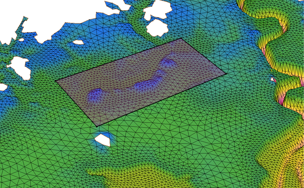
By aquaveo on April 2, 2024

Have you ever found yourself working on a mesh in the Surface-water Modeling System (SMS) that has holes in places you don’t want them? Then you may want to check out the new Fill Holes in UGrid tool in the SMS toolbox. This tool can be a quick and easy way to fill in any undesirable voids in your 2D mesh or unstructured grid (UGrid).

Example of a UGrid before using the Fill UGrid tool

The Fill Holes in UGrid tool can be found in the SMS toolbox under the Unstructured Grids folder. From there, all you need to do is select the mesh or UGrid that has holes or voids you want filled from a dropdown list, give the new mesh a name, and run the tool. From there, SMS will create a duplicate of the input mesh, only now the mesh will have elements where the holes used to be.

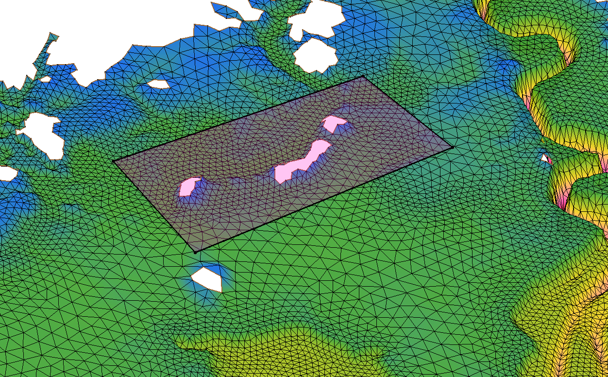
Example of a UGrid after using the Fill UGrid tool

But what if you want to keep some of the voids in your mesh? That’s where the Extract Subgrid tool comes in handy. The Extract Subgrid tool can isolate a portion of a mesh, which is useful if the mesh is particularly large, or if you want to confine any changes to one specific area.

To create a subgrid, first you need to create an Area Property coverage with a polygon outlining the area you want to isolate. Then open the toolbox and find the Extract Subgrid tool, which is located in the Unstructured Grids folder. Select the mesh from the “Grid” dropdown, the coverage from the “Subgrid boundary coverage” dropdown, and enter a name for the new mesh. Now you can use the Fill Holes in UGrid tool to fill the voids in just the isolated portion of the mesh.

If you use the subgrid method to fill the voids in your mesh, there is one more tool you’ll want to know about: the Merge 2D UGrids tool. You can use this tool to merge the subgrid back with the original mesh. This tool is also in the toolbox under the Unstructured Grids folder. To use this tool, select the subgrid from the “Primary grid” dropdown, the original mesh from the “Secondary grid” dropdown, and choose a name for the new mesh.

The Fill Holes in UGrid, Extract Subgrid, and Merge 2D UGrids tools can help simplify and smooth the mesh editing process, no matter the project. Open SMS 13.3 and check out what these three tools can do for you today!

Blog tags:

SMS

Using the Mask Subset Smoothing Option

By aquaveo on March 12, 2024

The Surface-water Modeling System now includes two new tools in the toolbox to help you when your project requires any amount of dataset smoothing. Previous versions of SMS had you use the Dataset Toolbox to smooth a dataset. These new tools can do everything that the Dataset Toolbox used to do, and more.

Both the Smooth Datasets and Smooth Datasets by Neighbor tools are used to eliminate extreme slopes in a dataset, but they require different inputs, which will tell SMS how to incorporate the relationship between nodes. The Smooth Datasets tool uses an anchor and either an elemental area change or maximum slope for its calculations. Smooth Datasets by Neighbor uses the relationship between neighboring nodes and a selected interpolation method: average or inverse distance weighted. Note that the current version of these tools are designed to be used on node-based datasets, so they will only work on a mesh.

Both of the dataset smoothing tools have the option to include a subset mask. A subset mask dataset is great if there are nodes or elements in your mesh that you don't want included in the smoothing process. Here's some things you need to know when using a subset mask in your project.

Before you begin making changes, your subset mask dataset needs to have the same number of values in the same locations as the dataset being smoothed. A simple way to do this is to right-click on the original dataset in the Project Explorer and select Duplicate. Then you can make changes to the duplicate to create your subset mask dataset.

All the nodes you want to have included in the smoothing process need to be set to an S value of "1.0", and the nodes that should be excluded need an S value of "0.0". You can do this in any way you'd like, as long as all nodes get assigned one value or the other. There is a quick method that you may consider using to assign these values. With the Select Mesh Node tool active, right-click in the Graphics Window and choose Select All. With all nodes selected, enter either "1.0" or "0.0" in the S value field depending on whether the majority of nodes should be included or excluded. Then manually select the nodes that should be excluded from the smoothing process by either clicking and dragging a box around the nodes, or by holding down the Shift key and selecting nodes, so that you can select multiple nodes at the same time.

Now this dataset is ready to be used as a subset mask. Open the tool's dialog and select the dataset from the Subset mask dataset dropdown in the tool dialog and enter any other necessary inputs, then run the tool.

To see all the changes, go to the Data menu, select Map Elevation, and select the new smoothed dataset. This will apply the changes that the smoothing tool made to the mesh in the Graphics Window.

Head over to SMS and try including a subset mask dataset with the Smooth Dataset tool today!

Blog tags:

SMS

Incorporating Rubble Mounds in CMS

By aquaveo on February 20, 2024

CMS-Flow and CMS-Wave are two of the principal components of the Coastal Modeling System. Rubble mounds are an important part of some coastal modeling projects. They are a common engineering structure used as jetties, breakwaters, seawalls, and groins for shoreline protection as well as flow and sediment transport control.

The way rubble mounds are implemented in the Surface-water Modeling System (SMS) is different depending on which CMS model you pick. Rubble mounds in CMS-Flow simulations focus primarily on sediment transport and morphology changes, while CMS-Wave focuses on wave processes. Both of these CMS models have their own coverages and sets of requirements in order to add rubble mounds to the project.

Rubble mounds can be added to CMS-Flow simulations through the CMS-Flow Rubble Mound Jetties coverage. Once this coverage is added, you can create a polygon in the Graphics Window that represents the rubble mound. Double-clicking on the rubble mound polygon opens the Rubble Mound Jetty Attributes dialog where you can define the parameters of the rubble mound structure. This dialog includes inputs for the name, the rock diameter, the porosity, the base depth, and the calculation method. After defining all the parameters, the coverage is ready to be added to the CMS-Flow simulation. Finally, make sure that Calculate sediment transport is turned on in the Model Control , otherwise your rubble mound is just a random polygon that has no effect on the final simulation.

Rubble mounds in CMS-Wave simulations work a little differently than CMS-Flow. CMS-Wave doesn't have a specific rubble mound coverage like CMS-Flow does. Instead, rubble mounds are defined on a CMS-Wave structures coverage. This behaves somewhat similarly to materials coverages that you may be familiar with in other SMS models. Double-click the polygon representing the rubble mound to bring up the Assign Structure dialog. Then you'll add a structure with the green plus sign, select "Rubble-mound" from the structures dropdown, and then whether or not you want to modify the rubble mound by elevation. If you'd like, you have the option of customizing the color and texture SMS will use to fill your polygon structure to something that best suits your project.

CMS-Flow and CMS-Wave each require their own simulations, but you have the option to couple them using inline steering. This is a great option if you're building a comprehensive coastal model.

Head over to SMS and try out adding rubble mounds to your CMS project today!

Blog tags:

SMS

Deciding between SRH-2D 2D Bridges and 3D Bridges

By aquaveo on February 6, 2024

In the Surface-water Modeling System, you have the option of adding either a 2D or a 3D bridge to your SRH-2D model. But what are the differences between 2D and 3D bridges, and how can you know which one is the best fit for your SMS project? There are pros and cons to each, so we will briefly explore each option, and hopefully by the end you’ll have a better idea of what works best for you.

Starting in SMS 13.3, the 3D Bridge component that was used in previous versions was retired in favor of 3D Structures. 3D Structures can be used to build 3D bridges as well as culverts, and can also be used to calculate overtopping, an option that wasn’t available with 3D Bridges.

For 2D bridges, you have many options to help you customize your bridge, such as setting the bridge width, type and number of piers, abutments, etc.. (For the full list, go to this page of our wiki). All of the options that exist for 2D bridges are also available when building a 3D bridge. Using the 3D structures coverage to build your bridge allows for even more customization, including being able to shape the bridge ceiling so there is variation rather than being a constant along the full length.You can also use the 3D structures dialog to add a UGrid to the Project Explorer so that you can see what the bridge will look like with the mesh. The 3D structures coverage dialogue is able to generate a mesh footprint for your bridge, which automatically includes voids in the mesh for your piers so you don’t have to create them manually.

If you have questions about the specifics of building a 3D bridge, check out the new 3D Structures tutorials, or our wiki page on 3D Structures to get a more thorough introduction.

Building a 3D bridge into your project is an excellent option when you want to go the extra mile with the visual representation of the bridge. Although the idea of using a 3D bridge for everything may sound great because of the extra visualization options, a 3D bridge isn’t going to be necessary, or even practical, for every project. SMS’s calculations will turn out the same regardless of which bridge type you pick. 2D bridges are often a better choice if you’re looking for just a quick representation for your bridge, or if you’re modeling multiple bridges at the same time. Having multiple 3D bridges can slow down the processing speed in a way that having multiple of their 2D counterparts wouldn’t.

Head over to SMS and try out the 2D and 3D bridge building tools in 13.3 today!

Blog tags:

SMS