Aquaveo & Water Resources Engineering News

Using the Blend Arcs Tool
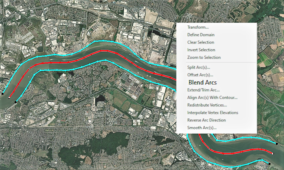
Sometimes it may be useful to have a quick way to create an arc that lies between two other arcs. For example, you might need to quickly create a centerline arc between two bank arcs. The Surface-water Modeling System's Blend Arcs tool, which is new to SMS in version 13.2, means that creating a blended arc is only a few clicks away.

There are many applications for the Blended Arc tool in SMS. As mentioned earlier, it can be used to find the centerline of a channel using the bank arcs. It can also be used for a quick way to find the arc in the center of a bridge, culvert, or weir.There are many other potential applications for this tool.

Example of the Blend Arc command

The steps to use the blended arc feature are:

  1. Create two arcs. The arcs can be parallel to each other, or even touching.
  2. After selecting both arcs, right-click in the graphics window and choose Blend Arcs from the menu.

The blended arc is immediately generated. This can only be done with two arcs, however the two arcs you pick don't have to be right next to each other. You can still find the blended point of two arcs that are separated by other features, such as other individual arcs or polygons.

When working around polygons in your project, If a polygon has been created in the space where the blended arc will appear, when the Blend Arcs tool is used, the polygon will retain its original shape despite the fact that there is now an arc splitting it. This could be useful for your project, but if you intend for the new arc to split the polygon into two new shapes, you only need to click the Build Polygons macro one more time and the new polygons will be created with this new division.

Try the new Blend Arcs tool in SMS 13.2 today!

Blog tags: 

Engineering with Nature in SMS

Aquaveo has joined in the Engineering with Nature (EWN) initiative started by the U.S. Army Corps of Engineers by adding Engineering with Nature tools into the Surface-water Modeling System (SMS). EWN aims to move toward a more efficient, sustainable, and resilient approach to engineering by considering social, environmental, and economic impacts. To support the mission of EWN initiative, SMS has developed multiple tools. Let's look at some of these tools.

Adding engineering features into your project can sometimes be a long and tedious process. With the EWN Features tool in SMS you can streamline the process, reducing the amount of time that would have been spent inputting the necessary data before. The EWN Features tool is built especially for creating feature objects to represent structures in natural environments. To use the tool, create a new map coverage and select the EWN Features type in the Engineering with Nature folder under the list of Model types to begin building structures into your SMS project.

Once you have a EWN Features coverage, you can create polygons to model the feature. You then can assign attributes and properties to the polygon. Once you have the feature properties defined, you can use the tools in the coverage to insert the define feature into a 2D mesh or 2D unstructured grid (UGrid).

Example of the EWN Polygon Properties

Another EWN tool is the Sediment Volume Management tool. The Sediment Volume Management tool allows you to calculate cut and fill for sediment volume. Like the EWN Feature tool, this tool is accessed by creating a new map coverage with the Sediment Volume Transport type found in the Engineering with Nature folder under the list of Model Types. In the coverage you can create polygons and assigned sediment parameters. Then the sediment volume calculations can be performed using the tools in the coverage.

Additional EWN tools are in development for SMS. Look for them in future releases of SMS. In the meantime, try out using EWN in SMS today!

Blog tags: 

Using Bias When Creating a 3D Grid

Sometimes when creating a 3D grid in the Ground-water Modeling System (GMS) you may want to include a bias in the grid for your project. Using a bias parameter will refine part of the grid along a particular axis. Here are some important things to know when implementing a bias into the grid.

All of the data fields necessary for this function will be in the Create Finite Difference Grid dialog window, which appears when a new grid is created. It is here that you can customize the X, Y, and Z-Dimensions to include your bias. The starting point for the bias is determined by the cell number designated in the Origin field of each dimension, and the bias will run along the axis in the positive direction. You can input a different value for the bias in each of the dimensions.

Example of the Create Finite Difference Grid dialog showing the bias option

For a value greater than one in the bias field, each cell will be a percentage larger than the one previous. For example, a bias of 1.2 will mean that each cell following the origin is 20 percent larger than the one previous. These cells will grow in the positive direction along the axis. To make each cell following the origin smaller than the one previous rather than larger, make the bias less than one. For example, a bias of 0.8 will mean that each cell will be 80 percent of the size of the previous cell.

Example of bias used on a 3D grid

The length field in each of the dimensions determines the total length of the dimension. All of the cells on that axis will fit inside that measurement. After specifying a length, there are two options for how GMS will calculate the size of the cells including the bias. First is by the number of cells in each axis. The grid creator will calculate how big each of the cells must be in order to fit that number into the specified length.

The second option for determining cell size is to input a value for the dimension of the starting cell. For example, setting the cell size to 10 feet will tell the grid creator that the origin cell should be 10 feet, and each cell following should be a percentage larger than the origin cell until the entire length of the axis is filled. This can be refined even farther by specifying a cell size limit, keeping a cell from growing larger than a specified size. Because of this, the cell size limit should be set to a number larger than the base cell size.

With GMS, there are many ways to customize a 3D grid. Give the grid bias function in GMS a try today!

Blog tags: 

Using NetCDF Data with AHGW Pro

Have you needed to use netCDF files with Arc Hydro Groundwater Pro? NetCDF files are intended to provide standardization to multidimensional scientific data. These files can be imported and used in ArcGIS Pro and are compatible with Arc Hydro Groundwater Pro. However, they must first be converted using ArcGIS Pro geoprocessing tools.

ArcGIS Pro has a few tools specifically dedicated to manifesting netCDF data as a familiar data form in ArcGIS Pro. These data forms include feature layers, rasters, and tables. Once netCDF data has been converted, it can be used with any Arc Hydro Groundwater Pro tool that accepts the given data form.

The ArcGIS Pro tools for netCDF data are found in the Multidimension Tools Toolbox. There's a toolset devoted to netCDF data, but some of the other tools in the Multidimension Tools toolbox will also work with netCDF data.

Example of ArcHydro Groundwater Pro greodatabase volume

The following is a suggested workflow for working with netCDF data and Arc Hydro Groundwater Pro:

  1. Use the appropriate tool from the Multidimension Tools toolbox to convert the netCDF data to the desired data form.
  2. If necessary, add it to the Arc Hydro Groundwater Pro geodatabase. This might be essential depending on what you hope to do with the data.
  3. Make any necessary adjustments or additions to the data to ensure compatibility with the Arc Hydro Groundwater Pro tool you hope to use.
  4. Use the feature layer, raster layer, and table view in the Arc Hydro Groundwater Pro tool of your choice.

A similar workflow exists for Arc Hydro Groundwater for ArcGIS Desktop:

  1. Load netCDF data into the map.
  2. Use the appropriate netCDF-related tool from the Multidimension toolbox.
  3. The output of that tool (e.g. a netCDF feature layer) can be used as input to any geoprocessing tool that accepts that kind of input.
  4. If desired, the temporary layer from the Make NetCDF Feature Layer tool can be saved to your computer's drive with the "Save To Layer File" or "Copy Features" tool.

It's possible that the netCDF data does not have the appropriate data for use with Arc Hydro Groundwater Pro. You might have to edit the data to ensure compatibility (e.g. adding HydroIDs). Furthermore, converting netCDF data to a feature layer or a raster does not mean you have all the data needed to run your Arc Hydro Groundwater Pro. Usually, the feature layer, raster layer, or table will just be one piece of running a tool effectively.

Try using netCDF data with Arc Hydro Groundwater Pro today!

Blog tags: 

Viewing SRH-2D Simulation Plots

SMS generates multiple plots during the SHR-2D model run. These solution plots include data collected by monitor points or lines as well as information such as mass balance and percentage of flow that enters the simulation. This post will discuss accessing and using the solution plots.

The first way to view the SRH-2D Solution plots is through the simulation data in the Simulation Run Queue. This allows you to look at the quality of the simulation as it is running. In the Simulation Run Queue, the Monitoring data option needs to be turned on. You can then view the plots as they are generated using the tabs below.

After you have run the simulation, you can view the solutions plots. You can access the SRH-2D Solution Plot by doing the following:

  1. Right-clicking on the simulation item and select Tools from the dropdown to open another submenu.
  2. Click on View Simulation Plots to pull up the SRH-2D Solution Plots window.

This will allow you to look at the list of different plots in the Plots section. On the left, there are a few other options such as the legend, and specifying the time range. The show legend option will have a legend appear in the upper right corner of the plot that has been pulled up. This as well as the specifying of the time range allows you to adjust the graph to your desired time range.

Example of the Solution Plots dialog

It is important to note that the plots in the Solution Plot window are not available in the Plot Wizard. You will need access them through the Solution Plots window. With that, it should be noted that pulling up an older SRH-2D project in a current version of SMS may not have the solution plots. This is because of changes in how files are organized. In this case, the solutions plots can be generated by re-running the simulation.

The SRH-2D Solution Plot is one of the many options in SMS to help you see what is happening in your simulation. Try using the SRH-2D Solution Plot in SMS today!

Blog tags: 

Working with Inactive Cells in MODFLOW 6

When working with a MODFLOW 6 model in the Groundwater Modeling System (GMS) it can be important to mark specific cells inside a project as inactive to keep it out of the computational domain. Using inactive cells can speed up the performance and accuracy of your model. Incorrectly designating cells as inactive or active can cause inaccuracies in your model or keep it from converging. Here is some guidance for working with inactive cells that will help create a better MODFLOW 6 model.

Modflow 6 model with inaccurate z values

When choosing which cells to mark as inactive in GMS, it is helpful to know how to find information about the cells in the first place, as well as what information MODFLOW 6 is using to calculate the X, Y, Z, and S values of that cell. The display above the graphics window that shows the values of the selected cell is using the cell center for its calculated values. If the inactive cells have a low elevation that is inaccurate for the model, it will drag the Z value for the active cells on the edge down to meet the inactive cell. This happens because the outside active cell has nodes in the Z value that still need something to attach to as there cannot be gaps between the nodes. This will distort the cells in unintended ways and create errors in the model.

MODFLOW 6 uses IBOUND to determine which cells to mark as active and which to mark as inactive. Marking a cell with an IBOUND value of zero will make it inactive.

There are a few ways to inactivate cells in a MODFLOW 6 model. The first is to create a polygon that will separate the active and inactive cells. Select the polygon that contains the cells that are to remain active. Go to the Feature Objects menu and select Activate Cells in Coverage(s). This will automatically make any cells that aren’t selective inactive.

The second way is to select a group of cells with the cell selection tool. Then go to the MODFLOW menu | Advanced | Cell Properties… and change the IBOUND dropdown menu to inactive. This will inactivate only the cells that have been selected in the graphics window.

The cells can also be set as inactive by editing the IBOUND Array directly.The IBOUND dialog can be found by clicking on Global Options under the MODFLOW menu. There is an IBOUND button in this dialog window where the IJK coordinates can be set to zero manually.

Making use of inactive cells can improve you MODFLOW 6 model. Try out MODFLOW 6 in GMS today!

Blog tags: 

Announcing WMS 11.2 Beta

Aquaveo is excited to announce the release of WMS 11.2 in beta! WMS continues to provide an all-in-one watershed modeling solution. With the release fo the WMS 11.2 beta, we want to highlight some of the new features you can find in WMS 11.2 beta.

WinTR-20 Model

WMS 11.2 has improved the use of the TR-20 model by incorporating the WinTR-20 numeric model. WinTR-20 uses the same interface as TR-20. WinTR-20 contains upgrades to the source code with some changes to the input and output files. These changes have now been incorporated into WMS 11.2 to let you take full advantage of these features.

Export MP4 Files

MP4 files are now the default when exporting animations. You can export the MP4 files directly from the film loop wizard in WMS. MP4 files make sharing animations you’ve created in WMS easier.

The Toolbox in WMS 11.2
Toolbox

WMS 11.2 introduces the Toolbox which contains many tools for manipulating data and geometries. This is reached through the Toolbox macro. Of particular use for WMS projects are the tools related to working with rasters and lidar data allowing to trim, merge, and smooth this data along with many other options. The toolbox also contains many tools for working with coverages and datasets.

Color Ramp Options

The final new feature is the changes to the color ramp options. The color ramp now contains multiple preloaded color palettes. Options have been added to reverse pallets and to save your favorite palettes for easy access in the future. The preloaded palettes can also be duplicated and customized to meet your project's needs.

These are a few of the new features that come out with the release of WMS 11.2. Try out these features and more by downloading WMS 11.2 from the Aquaveo website today!

Blog tags: 

Interpolating Localized Elevation Values

Do you have a Surface-water Modeling System (SMS) project where you need to adjust the elevation values for a small area of your mesh? Some projects require updates to the localized areas of the mesh elevation. It may be that you’ve received updated elevation data for part of the project area, or you discovered a flaw in the elevation data on the mesh. You could manually update the elevation on each node of the mesh, but this could be rather time-consuming. Using the Scatter Module in SMS, you can incorporate the new elevation values into your mesh.

Example of localized elevation data

Ideally, you will be able to obtain correct elevation data that covers the entire mesh domain, which you could simply interpolate over to the mesh. But when you only have updated elevation data for a localized area, you can use this workflow to update the elevation data.

  1. Right-click on the desired mesh and select Convert > Mesh → 2D Scatter.
  2. Name the new scatter set whatever you'd like (or keep the default) and keep all other settings the same.
  3. Choose Scatter | Merge Sets to open the Merge Scatter Sets dialog.
  4. Check the box for each scatter set that you would like to merge.
  5. Make your newer data higher on the list so that it will be given priority. Do so by selecting a scatter set and using the Move up or Move down buttons.
  6. Choose Delete lower priority scatter points and check the box for Maintain triangulation.
  7. If desired, name the new scatter set something other than the default.

This will create a new scatter set that overwrites the old data with the new data.

From here, which course you take will depend on whether you need just the z values to change, or if you need the mesh geometry to change as well.

To only change the elevation values in the existing mesh, do the following:

  1. Right-click on the new scatter set and select Interpolate to....
  2. Check the boxes for the scatter set z or elevation dataset as well as the box for Map Z.
  3. Choose the starting mesh from the list on the right.

To create a new mesh with the new elevation values, do this:

  1. Right-click on the merged scatter set and select Convert > | Scatter → 2D Mesh.
  2. Name the new mesh whatever you like and press OK.
  3. Edit the new mesh as needed.

The Scatter Module in SMS gives you a variety of options for fixing and adjusting elevation data. Try out the Scatter Module in SMS today!

Blog tags: 

Refining Quadtree Grids in SMS

Using the Surface-water Modeling System (SMS), you can model quadtree grids for use with numeric models such as CMS-Flow. Quadtrees are part of the UGrid module in SMS making them a type of unstructured grid. When creating quadtrees in SMS, you can choose to have uniform cell sizes, or you may choose to refine the cells in some areas. When refining a quadtree, there are a couple methods and some tips to keep in mind.

The first method for refinding grid cells in a quadtree is to simply select the cells you want to refine using the Select Elements tool, then right-click and use the Refine Cells(s) command. This will equally divide the cells into smaller, more refined, cells. This method is useful for small-scale refinement in localized areas. However, using this method can be tedious if there are multiple areas on the quadtree that need refinement.

Example of the Quadtree Refinement in GMS

The second method for refining quadtrees is preferred in most cases. This method involves setting refinement parameters in the Quadtree Generator coverage. If you are familiar with SMS’s Cartesian grid generator coverage and mesh generator coverage, you will find that it is similar to both of those coverages.

Like the Cartesian grid generator coverage, the quadtree coverage makes use of a grid frame to define the domain of the generated grid. In the grid frame, you decide the size of the cells in the generated quadtree. It is recommended that this cell size be the largest reasonable cell size for the quadtree grid.

Like the mesh generator coverage, the quadtree generator coverage also makes use of polygons. When you create a polygon on the quadtree generator coverage, you can double-click on the polygon to open the Polygon Attributes dialog. In this dialog you can set the grid cell size for all cells that will be within the polygon.

Using both the grid frame and the polygon attributes, you define how the grid cells are refined for your quadtree with more precision. Try out refining quadtree grid in SMS today!

Blog tags: 

Converting Between 2D and 3D Unstructured Grids

Many projects in the Groundwater Modeling System (GMS) start with an unstructured grid (UGrid). GMS supports both 2D and 3D UGrids. The type of UGrid you will need to use will depend on which numeric model you are using for your project. For this reason you may need to change a 2D UGrid to a 3D UGrid or vice versa. This blog post is going to review some of the tools for converting between 2D and 3D UGrids.

Typically, models like MODFLOW-USG or MODFLOW 6 will require a 3D UGrid. If you only have 2D UGrid data, this may require taking a 2D UGrid and converting it to be a 3D UGrid. Likewise, you may need to convert a 3D UGrid to be a 2D UGrid. This is more often done to correct uses with the 3D UGrid, but also to be able to use the data from the 3D UGrid with other applications.

GMS provides two tools in the Toolbox for changing between 2D and 3D UGrids: the Extrude to 3D UGrid tool and the UGrid 2D from UGrid 3D tool. The Toolbox is accessible through the Toolbox macro and these two tools are located with the Unstructured Grids tools.

Example of the Unstructured Grid tools in GMS

The Extrude to 3D UGrid tool converts a 2D UGrid to a 3D UGrid. The tool will allow you to select a 2D UGrid for extrusion, and then it lets you specify the number of layers and layer thickness for each of the new layers. This will extrude the 2D Ugrid to be a 3D UGrid with the specified number of layers that are at a uniform thickness. If you need layers to be at different thicknesses, you will need to edit the 3D UGrid using other tools in GMS.

The UGrid 2D from UGrid 3D tool will collapse a 3D UGrid to be a 2D UGrid. The tool allows you to select a 3D UGrid then select if the 2D UGrid should be created from the top or bottom of the 3D UGrid layers.

The unstructured grid tools in GMS allow you to have more options with how you work with UGrids and grid data for your groundwater projects. Try out the unstructured grid tools in GMS today!

Blog tags: 

Pages