Aquaveo & Water Resources Engineering News

Utilizing SMS's Gravity Waves Tools

Are you working with a coastal model in the Surface-water Modeling System (SMS) that includes a representation of how particles move through a mesh or grid? Did you know that the toolbox has Gravity Waves tools, which can help you visualize and find data about those particles more easily? This blog post will give you an overview of both the Gravity Waves Courant Number tool and the Gravity Waves Time Step tool and how they can help you with your ocean models such as ADCIRC.

Gravity Waves tools in the SMS Toolbox

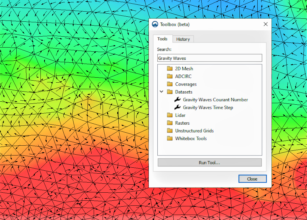
The Courant number is a value that represents the amount of time a particle stays in the cell of a mesh or grid. The purpose of the Gravity Wave Courant Number tool is to help maintain the stability of a numerical engine and, potentially, to help choose the most suitable time step measurement. If the methods used to solve numerical problems are restricted by the Courant condition, things can become unstable if the Courant number goes beyond the allowed limit. By looking at the highest Courant number in the dataset, you can get an idea of how stable the mesh is with respect to the chosen time step.

There are three necessary input parameters for the Gravity Waves Courant Number tool, the first being a dataset. This tool requires a dataset that represents the particle’s velocity magnitude. Second, you need to enter a gravity value. Lastly, you’ll enter a computational time step value. For the output parameters, you’ll choose a name for the new dataset. It should be something short and easily recognizable, possibly referencing the input dataset.

The Gravity Waves Time Step tool functions as somewhat the opposite of the Gravity Waves Courant Number tool. The purpose of the Gravity Waves Time Step tool is to calculate the time step needed to achieve the desired Courant number, based on the provided mesh and velocity field. You can then choose a time step for analysis that is equal to or greater than the highest value in the resulting dataset of time steps.

The required input parameters for the Gravity Waves Time Step tool are first, an input dataset, which should be set for depth. Note that it is important that the dataset is specifically for depth, not elevation. Second, enter a gravity value. Lastly, enter the Courant number you’re searching for. Choosing a value for the Courant number under the maximum threshold may increase the stability of the computation because the resulting computation is approximate. The output parameters are where you’ll specify a name for the new dataset. As with the Gravity Waves Courant Number tool, the name should be something short and descriptive.

Try out the Gravity Waves tools for yourself, and see what they can do for your SMS project today!

Blog tags: 

Calculate the Water Level Below the Top of an Aquifer

The Data Calculator is a useful feature that is available in the Groundwater Modeling System (GMS). The Data Calculator performs many functions and can enhance your project and simplify the visualization of data. This blog post will provide an overview of how to use the Data Calculator in GMS to pinpoint locations where the water level in a selected aquifer falls below the top elevation in a MODFLOW simulation.

Calculating the Water Level Below the Aquifer

As you might expect, a MODFLOW simulation containing aquifers needs to be completed before you are able to use the Data Calculator to find the time step where the water level falls lower than the top elevation in the simulation. The datasets required for this calculation are the top elevation dataset and the head dataset.

Before opening the Data Calculator, you will first need to duplicate the top elevation dataset. This is because the Data Calculator isn’t able to recognize the datasets directly under the MODFLOW simulation in the Project Explorer. Right-clicking on the top elevation dataset and selecting duplicate will create a copy of the dataset under the grid folder in the Project Explorer, and this duplicate can now be read into the calculator. If desired, you can right-click on the duplicate dataset and rename it to something that makes more sense to you.

The next step is to go to the Edit menu at the top of the screen and select Dataset Calculator to open the Data Calculator dialog. There is also a Data Calculator macro on the top row, which will bring up the same dialog. Follow these general steps to calculate the data once the Data Calculator is open:

  1. On the left side of the dialog, find and select the Head dataset.
  2. On the right side of the dialog, either select a specific time step from the list, or check the box that says “Use all time steps”.
  3. Click the “Add to Expression” button to add the Head data at the selected time steps to the calculation.
  4. Click the subtraction button (-), or use your keyboard to type the subtraction symbol.
  5. Select the copy you made of the top elevation dataset and click “Add to Expression”.
  6. In the Result field, enter a name for the new dataset.
  7. Press Compute, then click done to close the dialog.

After generating the new dataset, you can right-click on it in the Project Explorer and select “View Values”, which will let you view the data values for the selected time step. Any values denoted by a negative number indicate a water level lower than the highest point of the aquifer.

Head over to GMS and see the many ways the Data Calculator feature can be useful to you and your project!

Blog tags: 

Converting an Unprojected Raster to Vector Maps in SMS

In the field of hydraulic engineering, understanding flow dynamics in channels is crucial for effective design and analysis. Converting unprojected rasters with u and v components from a Large Eddy Simulation(LES) model to a vector map in the channel can provide valuable insights. However, this process can be challenging without the right workflow. In this post, we will explore one approach to achieve this in SMS.

  1. Preparing the Data
    To begin, project component rasters to the correct coordinate system. This ensures that the data is in the correct coordinate system for further processing. This can be done in SMS by importing the raster data in the GIS module. Then use the projection command
  2. Importing and Triangulating the Ugrid
    Next, drag the projected rasters in and convert the u component raster to a Ugrid format using the Raster to Grid tool in the toolbox for SMS 13.2. However, since the resulting Ugrid is created from a raster, the data points are not triangulated for proper interpolation. To address this, select the Ugrid in the project explorer and choose Cells | Triangulate. This allows the data to be interpolated across the surface accurately.
    Alternatively, you can create your own UGrid that encompasses the raster area. Make certain the UGrid has the correct projection.
  3. Incorporating Bankfull Channel Bathymetry
    To add the bankfull channel bathymetry from a raster, interpolate the bankfull elevation to the UGrid points. Use the Data | Map Elevation command to overwrite the existing Z dataset with values from the bankfull dataset. This step ensures that the bathymetry aligns with the UGrid for an accurate representation of the channel.
  4. Example of the Filter Dataset Values tool
  5. Displaying Vectors and Refining the Results
    After combining the u and v components, display the resultant vectors. However, it is common to encounter null vectors outside the channel, which may disrupt the visualization. To address this, utilize the filter and map activities in the dataset toolbox. These tools enable you to mask or remove the null vectors, ensuring a clean representation of the flow hydraulics in the channel.

By following this workflow, you can effectively convert unprojected rasters with components from an LES model to a vector map in the channel using SMS. Proper triangulation, incorporation of bathymetry data, and handling null vectors are critical for accurate visualization of flow dynamics. SMS proves to be a valuable tool in streamlining this process, empowering professionals to gain deeper insights into channel hydraulics and make informed decisions for various engineering applications.

Try out working with raster data in SMS today!

Blog tags: 

New Unstructured Grid Generation Tools in SMS 13.3

The Surface-water Modeling System (SMS) allows use of unstructured grid (UGrid) geometries with multiple numeric models. With that, we have been adding functionality to make generating UGrids easier and more convenient. The toolbox in SMS offers many tools to help speed up UGrid creation and simplify the process. SMS 13.3 beta offers the same tools as before, as well as some new ones. As of now there are fifteen tools under the Unstructured Grids folder in the toolbox. The tool types cover conversion from different types of data to a UGrid, import and export tools, and more. This blog post will explore just two of the many different options in the toolbox.

UGrid creation tools in SMS 13.3

The first UGrid creation tool we will explore in this blog post is the UGrid from Coverage tool. The UGrid from Coverage tool takes the feature objects on a selected coverage and generates a UGrid from the properties of those feature objects. The tool can work with multiple coverage types. Like using the mesh generator coverage to create 2D meshes, the spacing of vertices on the arcs will determine the refinement of the generated UGrid. To generate a UGrid, the coverage must have at least one polygon in it. The parameters required when executing the tool are a coverage, and a name for the new UGrid. We recommend choosing a name that is short, but references the input data for easy reference.

The second UGrid tool we will explore is the UGrid from Surface tool. The UGrid from Surface tool takes an existing mesh, scatter set, or Cartesian grid and creates a new UGrid with copies of all of the datasets. This can be useful because it changes the data into a form that can be modified and manipulated while still preserving the original data. The input parameters include an input mesh, scatter set, or Cartesian grid, and an output grid name. Again, we recommend choosing a name that is short and references the input data.

All of the UGrid tools are accessible by clicking on the toolbox macro at the top of the window, then expanding the Unstructured Grids folder.

Download the SMS 13.3 beta and explore how the UGrid from Coverage and UGrid from surface tools, as well as the numerous other UGrid tools, can help your project today!

Blog tags: 

Understanding the MODFLOW Translator

When importing a MODFLOW file into Groundwater Modeling System (GMS), you may need to translate the file to ensure compatibility with GMS's features and tools. This blog post includes details about the versions of MODFLOW supported by GMS, how GMS uses the translator dialog to transform the MODFLOW file into a version that GMS is able to read and alter, and methods you can use to determine the file version.

Example of the MODFLOW Translator

GMS supports MODFLOW versions 88, 96, 2000, 2005, MODFLOW-NWT, MODFLOW LGR, and MODFLOW USG. However, MODFLOW 88 and 96 are only supported as imports and require conversion to MODFLOW 2000. When importing a MODFLOW file into GMS, if the file was not created in GMS 6.5 or later, translation is necessary for full compatibility with GMS's features and tools, so the MODFLOW Translator dialog will appear. GMS will create a copy of the file before performing the translation which will ensure that the original file is preserved, however you should still always double check that all the data was converted successfully and hasn’t been changed and that none of the data has been lost. During the translation process, you can select the appropriate MODFLOW version from the list provided by the translator for accurate interpretation and conversion.

You can also alter the MODFLOW version inside GMS between supported versions by going to Global Options under the MODFLOW menu. It should be noted, however, that while most versions can be changed back and forth, it can’t be changed back from MODFLOW USG Transport.

There are specific indicators for each version of MODFLOW that can help you to determine what kind of MODFLOW file you are working with if you are unsure which file type it is, which you can view by opening the file as a text file. In a MODFLOW 88 file, the third line of the basic package file contains an IUNIT array with 12 or 24 slots, 24 being the more common option. A MODFLOW 96 file, on the other hand, lacks the IUNIT array and instead features the keyword "FREE" on the third line, indicating that data is in free format, or the third line is entirely blank. Files with a *.dis extension are likely to be MODFLOW 2000, 2005, or NWT models, all of which are supported by GMS.

Certain features and versions of MODFLOW are not supported in GMS. If you have more questions about what MODFLOW features are not supported by GMS, you can follow this link to Aquaveo’s wiki for more information. Head over to GMS and see how this can work for your own MODFLOW models today!

Blog tags: 

Combining Runoff in Watershed Basins with WMS

The Watershed Modelling System (WMS) includes use of the Rational Method, which enables the calculation of peak flows for small watersheds in urban and rural areas. This feature can combine runoff from multiple basins to find the values.

The Rational Method requires a couple specific components to calculate the runoff coefficient for an area. The required inputs are soil data, along with either a table relating soil IDs to runoff coefficients, or a runoff coefficient coverage. Composite runoff coefficients use an area-weighted average of all runoff coefficients that overlay each basin for computation. The inputs chosen will depend on what method you choose to calculate runoff in the Rational Method module. The two primary methods to calculate runoff are first, to assign coefficients to polygons within a coverage, and second, to import a table with all of the coefficients already assigned to a land or soil use ID.

Example of Land Use in WMS Example of Soil Group in WMS

There are two ways to assign runoff coefficients to a polygon. The first way is to enter the coefficients polygon by polygon, and the second is to assign the coefficients through the Soil type mapping dialog.

To assign runoff coefficients polygon by polygon, do the following:

  1. Start with a Runoff Coefficient coverage.
  2. Select one of the polygons that intersects the drainage basin.
  3. Enter the runoff coefficient that matches the soil or land type for that polygon in the Runoff Coefficient dialog window that appears.
  4. After entering the data for each polygon that intersects the basin, activate the Hydrologic Modeling Module and go to Calculators | Compute GIS Attributes.
  5. In the Compute GIS Attributes dialog, make sure the following options are active:
    • “WMS Coverages” is selected as the data type.
    • Under Computation, Runoff coefficients is selected on the dropdown menu.
    • The “Use” dropdown is set to runoff coefficient coverage.
    • The “coverage name” dropdown is set to your new coverage.

To assign runoff coefficients to polygons by soil mapping, do the following:

  1. Start with a “Soil Type” coverage.
  2. Select one of the polygons that intersects the drainage basin.
  3. On the bottom left of the Soil type mapping dialog that appears, turn off the "SCS Soil Type" checkbox and turn on the "Runoff Coefficient" checkbox.
  4. You will now have a list of soil IDs and names with a field for runoff coefficients. Enter a coefficient value for each of these fields according to the material type.
  5. Open the Compute GIS Attributes dialog as described above.
  6. Set everything the same as are in the last set of steps, except change the "Use" dropdown to Coverage.

There are multiple ways to create runoff coefficient tables to import into a project. One of the ways is to create a table from scratch. If you choose this route, you can view the structure requirements on the Aquaveo wiki to make sure it includes everything you need. To import a table with the runoff coefficients, do the following:

  1. With the “Soil Type” coverage active, double-click on a polygon that intersects the drainage basin.
  2. Select “Import file” under Import soil attribute file.

You can also import a table in the Compute GIS Attributes dialog.

Head over to WMS and try out the different ways to assign runoff coefficients to your watershed project today!

Blog tags: 

Announcing SMS 13.3 Beta

Our developers have been hard at work making improvements and expanding the functionality of SMS. Aquaveo is happy to announce the release of the beta version of SMS 13.3!

To show you some of the things you'll see in this version of SMS, we've compiled a short list of some of the new features included in this release.

Improvements to SRH-2D

In SMS 13.3 beta, we have added support for the use of unstructured grids (UGrids) in SRH-2D modeling and simulations in addition to meshes. SRH-2D also now supports the use of DIP files in its modeling, and we updated the scour calculator. We also updated the model execution to eliminate false positives and SRH-2D will only call HY-8 one time when running multiple simulations which removes the possibility of collisions.

Changes in the Toolbox

If you visit the Toolbox in SMS 13.3 beta, you'll find that it has been reorganized and some of the naming conventions have been changed, as well as an added folder for 2D Mesh tools. If you can't find a tool that you've used in previous versions, don't worry. All the same tools are available to you, it may just be under a slightly different name or in a different folder.

New Tools

There are also several new tool options in the Toolbox. This includes, but is not limited to:

  • Polygons from UGrid Boundary: converts the outer boundary of a UGrid to polygons in a new coverage. This tool only functions on UGrids with 2D Cells.
  • Fill Holes in UGrid: fills all voids in a given mesh with new mesh elements. The output is a mesh that can be converted back into a UGrid if needed. This tool also works on meshes.
  • Refine UGrid: create a 2D UGrid that has been refined based on an existing 2D UGrid and one or more elevation rasters.
  • Curvilinear Grid tools: import and export a curvilinear grid in the form of a CH3D or EFDC file.
Example of the Smooth UGrid Tool in SMS

As always, the help button in the tool dialog will direct you to a page on our wiki that will give you a more thorough description of the tool and its function.

The Community Edition of SMS 13.3

One of the major changes in SMS 13.3 beta is that we have made four models available in the free community edition of SMS. New models that are now included in the community editions are:

  • ADCIRC (ADvanced CIRCulation): a hydrodynamic model used for modeling oceans, inlets, rivers, and floodplains.
  • AdH (Adaptive Hydraulics): a model used for groundwater and overland flow.
  • CMS-Flow: used for more local modeling, mainly for inlets, the nearshore, and bays.
  • STWAVE (STeady State Spectral WAVE): models wave refraction, shoaling, breaking, diffraction, wind-driven wave growth, and wave-wave interaction with energy redistribution and dissipation.

These are only a few of the new features offered in SMS 13.3 beta. You can find the list of all new features on this page of our wiki. Try out SMS 13.3 by downloading it today!

Blog tags: 

Selecting the Right MODFLOW Solver Package

Have you wondered which MODFLOW solver to use for your MODFLOW project in the Groundwater Modeling System (GMS)? When creating a groundwater model in GMS using MODFLOW, the selection of the solver package is an important decision that will affect the accuracy, speed, and efficiency of your model. This post will cover different complexities to consider while using GMS for your project.

Example of MODFLOW Solvers available in GMS

MODFLOW offers different solver packages, and the appropriate selection depends on the specific characteristics of your model. Here are some tips and ideas on how to select a solver package for your MODFLOW project in GMS:

  • Consider the size and complexity of your model. Some solver packages are more suitable for large and complex models, while others are better for smaller and simpler models.
  • Look at the type of boundary conditions you are using. Some solver packages are more appropriate for models with sharp contrasts in hydraulic conductivity, while others are better for models with more gradual changes.
  • Consider the amount of memory available on your computer. Some solver packages require more memory than others, and this can affect the size of the model you can simulate.
  • Look at the speed of the solver. Some solver packages are faster than others, but this may come at the expense of accuracy.
  • Consider the level of expertise you have with the solver package. Some solver packages are more user-friendly than others, and require less knowledge to set up and run.

Here are some general pros and cons of the available solver packages in MODFLOW:

  • PCG - this is the most commonly used solver package in MODFLOW. It is versatile and can handle a wide range of models. It is efficient for small to medium-sized models. However, it can be slow and memory-intensive for larger models.
  • GMG - this solver package is suitable for models with irregular grids and can handle models with steep gradients in hydraulic conductivity. It is efficient and requires less memory than PCG. However, it can be slower than PCG for models with smoother gradients.
  • LMG - this solver package is designed for large-scale models with highly heterogeneous geology. It is efficient and can handle models with multiple stress periods. However, it requires more memory than PCG and can be slower for smaller models.
  • NWT - this solver package is suitable for models with nonlinearities and can handle models with large gradients in hydraulic conductivity. It is efficient and requires less memory than PCG. However, it may be less accurate than PCG for models with sharp contrasts in hydraulic conductivity.

In summary, selecting the appropriate solver package for your groundwater model in MODFLOW requires careful consideration of the size, complexity, and boundary conditions of your model, as well as the amount of memory available on your computer, the speed of the solver, and your level of expertise with the solver package. Using GMS makes it easier to see which MODFLOW solver is best suited for your project. GMS also prevents selecting MODFLOW solvers that are incompatible with the selected version of MODFLOW.

Try out using the different MODFLOW solvers in GMS today!

Blog tags: 

Troubleshooting an SRH-2D Model

Do you have an SRH-2D model that is failing to converge or has other errors? It is important to understand that errors in SRH-2D model runs are not uncommon and not necessarily an indication of a major problem. This post will give you some guidance so you can quickly identify and fix errors. This will allow you to produce accurate and useful results.

Common errors often appear around items that were missed during the model development. To avoid errors, it is important to review all data that’s been important into SMS. Also, care should be taken in designing and generating the mesh or grid being used in the simulation. While SRH-2D is rather forgiving, sometimes small issues in the mesh or grid can cause errors. Finally, double-check all boundary conditions that they are in the correct location and that all model parameters have been set.

It's important to note that while the SMS model checker can identify some errors, it does not validate the data and cannot catch all errors. Therefore, it is important to be familiar with the SRH-2D error codes and how to troubleshoot them.

Example of error found in an SRH-2D project

When encountering an error, it is important to remain calm and follow the steps outlined in the blog post, recording the error number and referring to the SRH-2D error page for guidance. Often, solutions involve minor adjustments to data inputs or boundary conditions.

If you were unable to record the error from the model wrapper, don't worry. You can still see this information by reviewing two of the files generated by SRH-2D during every model run. These files will be named [projectname].OUT.dat and [projectname].DIA.dat files.

To use these files:

  1. Locate the files in the model run directory with your project file.
  2. Open the *.OUT.dat or *.DIA.dat files using a text editor such as Notepad.
  3. Look through the text file to locate the error code.
  4. Go to the SRH-2D error page to find the solution.
  5. Make the needed change(s) to your project and run SRH-2D again.

By mastering the process of troubleshooting SRH-2D errors, you can produce accurate and useful results that can inform important decisions related to water resources and hydraulic engineering. The Community Edition of SMS is a great resource for exploring the capabilities of SRH-2D in SMS. Use SRH-2D with SMS today!

A previous version of this article was publish in 2018

Blog tags: 

Fixing Negative Water Depth

If you've worked with an SRH-2D model in the Surface-water Modeling System (SMS), you may have noticed that there will be times that some nodes appear to have a negative water depth. This can be problematic because it often doesn't reflect the true nature of the body of water. SRH-2D simulations default their calculations to be cell-centered, while meshes calculate data from the nodes. Inactive cells are set to have a null value of -999, but if you're working with meshes, the nodes that touch the inactive cells will interpolate with the value of -999, thus causing a negative water depth to generate on that node. If this is something you want to avoid, here are some ways to eliminate a negative water depth.

Example of negative depths in an SRH-2D project

The first way to eliminate these negative water depth values from your SRH model when working with a mesh is to run your simulation as normal, and then use the Data Calculator in the Data Set Toolbox to truncate the data to a more desirable number, often this number will be zero. Follow these steps to truncate the data:

  1. Open the Data Set Toolbox under the Data menu.
  2. Under the Math section, select the Data Calculator.
  3. Find the dataset you are wanting to truncate, which will be labeled with "d#".
  4. Enter the following formula into the Calculator: "trunc(x,a,b)" where x is the dataset to be truncated, and where all the data will be greater than or equal to a, and less than or equal to b.
  5. Change the Output dataset name to one that suits your project.
  6. Click Compute, then close the Data Set Toolbox.

Make the new truncated dataset active in the Project Explorer, and note that the new minimum water depth is zero.

Example of truncated values in an SRH-2D project

Another way to get rid of negative water depths is to use an unstructured grid (UGrid). Ugrids use the same cell centered calculations that SRH-2D does, so you won't run into the same issues with how the data is interpolated. If you have already created your simulation on a mesh, you can follow these steps to convert to a UGrid:

  1. In the Project Explorer, right-click the desired mesh and select Convert | Mesh → Ugrid.
  2. If desired, change the Output grid name to something that suits your project.
  3. Remove the mesh from the simulation by right-clicking on the mesh name under the SRH-2D Simulations folder and selecting Remove.
  4. Drag the newly converted UGrid under Sim in the SRH-2D Simulations folder.
  5. Run the simulation again.

SRH has now recalculated the data with the UGrid with only cell-centered interpolation, which should remove any unintended negative water depth calculations.

Go to SMS and try out these ways to eliminate negative water depth today!

Blog tags: 

Pages