Aquaveo & Water Resources Engineering News

3 New Features in GMS 10.5 Beta

We are happy to be announcing the beta release of GMS 10.5! Thanks to the hardworking developers here at Aquaveo there are a number of new and exciting features to this new version.

To name a few, we gathered a list of three new and improved features in GMS 10.5 beta release!

  1. MODFLOW 6 Grid Approach
    Additional functionality has been added for working with MODFLOW 6. A MODFLOW 6 model can now be built in GMS using the grid approach. The new MODFLOW 6 interface uses a simulation approach that is different from the interface for other MODFLOW applications in GMS. This approach also allows for multiple simulations to be included in a single project.
  2. TVM Package
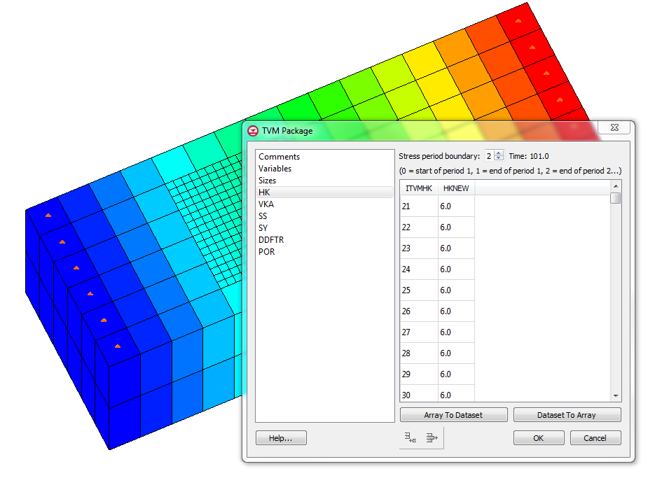
    The TVM package is now available in GMS 10.5 for use with MODFLOW-USG Transport. The Time-Variant Materials (TVM) package allows the changing of hydraulic conductivity and storage values between stress periods. Through a transient simulation, it can also be used to change these parameters in a continuous manner not just in increments between stress periods. This will help display the different changes made to the project over time.
  3. TVM Package in GMS 10.5
  4. Tile map services (TMS) can now be used for import or background image display.
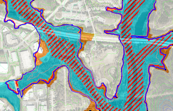
    In this new version of GMS the ability to import TMS into projects needing tile map services has been made available. This provides access to maps that can now be rendered to map tiles at fixed scales. Rather than trying to break down one large image, this helps to be able to view a map in a simpler way. It also helps to be able to pinpoint and save one particular tile of a map in case only that tile is needed as opposed to the entire image.

These are only some of the changes that have been made to the new beta release version of GMS. Explore even more of the changes by downloading GMS 10.5 beta from our downloads page.

Blog tags: 

Tethys Training in Kenya

Aquaveo was recently given the opportunity by NASA SERVIR to develop a training course involving the Tethys Platform. NASA SERVIR is a joint venture between NASA and the U.S. Agency for International Development.

RCMRD Building

SERVIR works to provide better informative forecasts regarding the risks of floods as well as an outline of what happens after the devastation of flooding in an area. Thus, it was exciting to participate in furthering their mission to provide state-of-the-art, satellite-based, and Earth monitoring data.

In partnership with NASA SERVIR, Aquaveo led in developing and delivering training courses on app development through the use of the Tethys Platform. The Tethys Platform provides a suite of free software which helps in creating water resource applications. Due to the unique system Tethys uses, less code and written HTML is needed for the development of applications. These are just a couple of things that make the Tethys Platform a useful resource for web developers.

From February 24th to the 28th, twenty-one individuals from Ghana, Senegal, Nepal, Columbia, Peru, USA, and Kenya traveled to the SERVIR Eastern and Southern Africa Hub at the Regional Centre for Mapping of Resources for Development (RCMRD), located in Naribi, Kenya to attend both a communicative and individualized training.

Tethy training in Kenya

The Regional Centre For Mapping Resource For Development has been dedicated to promoting sustainability through the use of GEO-information. Their aid in supplying tools and space for Aquaveo to lead a training on the Tethys Platform was another step toward promoting sustainable development world wide. After four days of training, each participant left with even more knowledge on app development and will in turn further the progress in the Regional Centre for Mapping of Resources for Development's (RCMRD's) mission.

Tethy training in Kenya

The majority of the training focused showing how to develop applications using the Tethys Platform. Each contributor also took part in a more individualized training where one of the four training days was entirely dedicated toward working on and receiving help with their own personal projects. Aquaveo enjoyed the time spent working with these amazing participants and can’t wait to do it again.

Two additional training courses will be provided by Aquaveo within the year. We have the opportunity to meet more participants and lead a training in the areas of Kathmandu, Nepal and Huntsville, Alabama.

Experience learning more about Tethys Platform app development and keep an eye out for more details about future training courses!

Blog tags: 

Tips for Sharing SRH-2D Project Files

In SMS, projects are saved out as a series of files. These files should be kept together when sending a project to a coworker or associate. The exact files needed often varies based on the numeric model being used. This article will discuss the files needed when sharing an SRH-2D project.

There are a few items to keep in mind when sharing your SRH-2D project files.

Make certain all of the files have been included when sending them to someone else. The core files that are generally needed include:

  • SMS project file (*.sms)
  • Map data file (*.map)
  • Mesh data file (*_meshes.h5)
  • Materials data file (*.materials)
  • Any GIS or image files such as TIFs, JPGs, or shapefiles

One of the easier ways to make certain all of these files are included, is to use the Save As Package menu command. This command is found in the File menu. Using this command will place all of the files listed above into a single ZIP file.

The Save As Package command
Solution Files
If you have already run SHR-2D and have solution files, these files should be included with the other files. When opening the project file, sometimes the solution files will not be visible. To import the SRH-2D solution, select the Open command, then locate the *_XMDF.h5 file and import it into the project.
HY-8 Culverts

When sharing an SRH-2D project that includes HY-8 culverts, be certain to include the HY-8 file. It also may be necessary for the person receiving the files to relaunch HY-8 before running SRH-2D again. This is done by doing the following:

  1. Right-click on the boundary condition coverage containing the culvert and select the HY-8 Options menu command.
  2. Select the HY-8 file.
  3. Select the HY-8 arcs, then right-click and select the Assign Linear BC command.
  4. Launch HY-8.
Restart Files

If the project used a restart file, be certain to also include the *.rst file with the project. In some cases, this file needs to be specified again in the SRH-2D Model Control dialog before running SRH-2D.

Keeping track of all of the files necessary for an SRH-2D project makes certain the project can be used by anyone. Explore SRH-2D and other models in SMS today!

Blog tags: 

Tips for Using the Data Calculator in GMS

The Data Calculator in GMS is a powerful tool that allows you to generate new datasets from existing data.

The Data Calculator can be used to to create datasets that show:

  • The difference between model runs
  • The minimum or maximum of two datasets
  • An aquifer's water level
  • And many other applications

To help you get the most out of the Data Calculator, here are some tips for using this tool.

Datasets can be added to the expression by either double-clicking the dataset in the Dataset section of the calculator, or selecting the dataset and using the Add to Expression button. Make certain you are selecting the correct dataset before adding it to the expression.

When adding operators to the expression, be careful. Double-clicking the operator buttons will enter the operator into the expression twice. If this happens, be sure to delete the additional operator before computing the dataset.

Operators in the Data Calculator

Review datasets before using them in the Data Calculator. This can be done before starting the Data Calculator by using any of the available tools in GMS. Once in the Data Calculator, you can review datasets by selecting the dataset and clicking the Dataset Info button.

When adding a dataset to the calculation, either specific time steps can be used or all time steps can be used. When using specific time steps, select the desired time steps before adding the dataset to the equation, or enter the dataset number followed by a colon and the number of the time step.

Using a specific time step is the default option. To use all the time steps, select Use all time steps before adding the dataset to the expression, or enter the dataset number followed by a colon and the word "all".

Now that you know a little more about the Data Calculator, try it out with your projects in GMS today!

Blog tags: 

Using Command Line Switches for the XMS Installer

If you work as a system administrator or in an IT department, you may need to know how to install GMS, SMS or WMS silently or with less visibility. Fortunately, we have a few options for this.

Previously we have discussed performing a silent install of XMS, this article will discuss options that run as command line switches. For example, when running the WMS 11.0.5 installer with no UI, you will enter the command "wms11.0.5full64bit.exe/qn" through cmd.

When installing XMS, you have the following parameters you can set:

full UI: /qf

This is the default parameter used by the installer. This means that the end user will see the full installation wizard the same way they would by running it through Windows Explorer.

reduced UI: /qr The user interface does not show any wizard dialogues.

This is a form of automatic installation that will skip all wizard dialogues, though you will still see a full UI showing that WMS is being installed.

basic UI: /qb Only a progress bar will be shown during the installation

Command line install progress bar

This option is similar to /qr but, instead of showing the full UI from our installer, it shows a progress bar with default Windows installer decorations. This takes less screen real estate while still giving you visibility into the installation process.

no UI: /qn No UI will be shown during the installation.

This option does not show any UI at all, instead opting to run the install progress in the background. This is ideal for if you are installing the software on a computer that's currently in use and don’t want to interrupt the work currently being done.

Current versions of XMS software can be found on Aquaveo's downloads page.

Blog tags: 

Utilizing Data Modification Tools in SMS

The Dataset Toolbox in SMS allows viewing your data in many different ways, while also being used to modify and create new datasets from already existing datasets. The different tools in the toolbox each use a specific set of functions to modify selected datasets.

One tool in the Dataset Toolbox that can prove to be helpful is the Filter tool. This tool creates a new dataset based on the selected filtering criteria.

For example, say you are filtering your numeric model output to show depths between the minimum and maximum depth, then you wish to filter the depth data for velocity between minimum and maximum range. This tool could help to show how a fish habitat changes over time or for any other purpose you can think of.

There may be multiple ways to accomplish this task, but one method would be to filter the velocity dataset to the desired range and then map that activity to the depth dataset. Using this example, you could do the following:

  1. Open the Dataset Toolbox.
  2. Select the Filter tool.
  3. Use the tool to filter the Velocity Mag dataset to the desired range and apply NULL outside the range.
The Filter tool in the Dataset Toolbox

The Map Activity tool is another tool that can be helpful. This tool maps the activity from one dataset to a second dataset. It helps show only the values of interest on a particular dataset. To continue the previous example:

  1. Select the Map Activity tool in the Dataset Toolbox.
  2. Using the dataset created in the previous steps, map the activity from the new dataset to the depth dataset (Value Dataset).

The new dataset will appear in the Project Explorer, showing the values of interest. If the dataset is a transient then a film loop could be made, showing how it changes over time.

The Filter and Map Activity tools are only two of many tools available in SMS’s Dataset Toolbox. Try out these tools and others in SMS today!

Blog tags: 

Exploring Hide, Show, and Isolate in GMS

Many projects in GMS can end up being visually busy. Having a large grid and dozens of features can make it hard to see specific areas clearly. To help with this, GMS provides the Hide, Show, and Isolate functions.

How to Hide Cells

This feature allows you to select different project cells and simultaneously hide them from view in the Graphics Window.

  1. Select the individual, or group of cells that need to be hidden.
  2. Once it is highlighted, click the Hide macro in the toolbar, or right-click and select the Hide command.

Remember that when cells are hidden from view this does not mean they have been deleted from your project entirely. Even if they are not visible it is only necessary to select the Show macro on the toolbar and the hidden cells will reappear.

Also, hiding cells does not make those cells inactive. They will still be included in your model run.

How to Show Cells

To reverse the hidden elements, click the Show macro in the toolbar and any hidden cells in your project will reappear. This can be important if you have inherited a project and suspect there are hidden cells.

Isolating Cells

Isolating cells hides cells that are not selected, unlike Hide which hides the selected cells. To isolate cells:

  1. Select the cells in the Graphics Window you wish to isolate.
  2. Once cells are highlighted, select the Isolate macro on the toolbar, or right-click and select the Isolate command.

Using a Polygon

Another option for isolating or hiding cells is to use a polygon in the map coverage. To do this:

  1. Right-click on the selected polygon.
  2. Click Select Intersecting Objects from the menu that appears.
  3. In the Select Objects of Type dialog choose the geometric object to use.
  4. With the cells selected, you can now use the Hide or Isolate function.
Isolating cells using a polygon

Try using the Hide, Show, and Isolate features in GMS today!

Blog tags: 

4 Ways to Screen Capture in WMS

Are you needing to capture a screenshot of your WMS model? Fortunately, there are multiple ways to get a screenshot from WMS. This blog article will discuss four methods for using screen capture in WMS; two that use built-in Microsoft Windows capabilities and two that make use of the innate capacity of WMS.

Windows Methods

Microsoft Windows has a couple of innate methods for making a screen capture. One way is to use the Print Screen command found on the keyboard. This command will copy an image of the WMS screen into the computer's memory where the image can later be pasted into another program. Holding down the Alt key while using the Print Screen command method will limit the image to just the WMS interface if it is in the active window. This method, however, has one disadvantage considering that the captured image often needs editing.

Another method is to use the Snip tool. This tool initiates dragging a rectangle around the WMS interface. Like the Print Screen key, this saves the image in your computer’s memory which later needs to be pasted into a seperate program. This method has the advantage of allowing you to get a cropped version of the image.

Neither of the screen capture methods using the native Windows tools directly results in a usable image file.

WMS Methods

Using the WMS screen capture methods, a usable image file can be easily obtained. The Save As command and the Screen Capture command both create an image file that contains exactly what is displayed in the Graphics Window at the time the file is saved. This can help avoid having to copy and edit the image in a graphics software program.

To use the Save as command, go to File | Save As. In the Save As dialog, change the file type to be "JPEG Image File (*.jpg, *.jpeg)".

To use the Screen Capture command, make the GIS module active. Use the Image | Screen Capture command. In the save dialog that appears, save out the screen capture as a bitmap image.

Screen Capture command

Try out the screen capture capabilities of WMS today!

Blog tags: 

Viewing Flood Extents in SMS

For many riverine projects, finding areas of potential flooding is a key component. SMS offers a few ways to see the flood extents in a given project.

When running a riverine numeric model, such as SRH-2D, a dataset of the water surface elevation (WSE) is often part of the resulting solution. Using the contours and time steps of the WSE dataset can help locate the flooded areas and extents within the modeled area.

You can use the “max” function in the data calculator to make a dataset showing the maximum water surface elevation across all timesteps. For example, using a WSE dataset, you would enter "max(WSE:all)" to get the maximum value for the WSE dataset across all time steps. This would then show the maximum extents.

A faster way to view floodplain data for a single time step is to use the Map Flood command. This tool utilizes ground elevations and existing flood hazard maps from the Federal Emergency Management Agency (FEMA) to quickly visualize the impacts of possible modifications in the flood level. The Map Flood tool works with FEMA flood hazard data allowing you to avoid building and running an entire numeric model in order to obtain a quick estimate of the flood areas for a single time step.

Flood Extents using Map Flood

The Map Flood tool can also be used for a single time step with local data for areas where FEMA data is not available. More information about the Map Flood tool is found in the Fast Floodplain tutorial.

You can share the flood data you’ve generated by exporting a WSE or max WSE dataset in a variety of file formats using either the right-click Export command or the File | Save As command. The feature arcs created using the Map Flood can also be saved as a shapefile or any other available file format.

Try out the tools in SMS for viewing flood extents today.

Blog tags: 

Sharing Display Themes in GMS

Display themes make showing off your groundwater model easier. A display theme is a set display parameters that can be saved in a project to be used repeatedly. But, after creating a display theme that works well, have you ever wanted to use that same display theme for a different project?

Display Theme Example

In GMS, display themes are saved with the project file. Therefore, importing a display theme into another project isn’t quite as simple as importing a raster file or image. However, the process isn’t all that complicated either.

To import a display theme from an existing project into a new project, do the following:

  1. Open the project with the display theme you want to import to other projects.
  2. Remove everything from the project except for the desired display theme.
  3. Use the Save As command to save the project with a different name. The project should only contain the display theme.
  4. Open the project that is to receive the display theme.
  5. Select the File | Open command.
  6. In the Open dialog, select the project containing the display theme and turn on the Import into current project option before clicking the Open button.

Using these steps will add the display theme to the existing project. The new display theme will appear in the Project Explorer.

Note that this project requires using the File | Open method of importing a file. The Open macro can also be used. Other methods for importing files into GMS, such as drag-and-drop, will not work.

Also, be aware that when importing a display theme into an existing project, the display theme will only work with data like that in the original project. For example, a display theme built for a project using 3D UGrids will not work with a project that uses 2D grids.

Display themes are a great tool for visualizing your data in GMS. Try saving and sharing them in GMS today!

Blog tags: 

Pages