Aquaveo & Water Resources Engineering News

Troubleshooting TOPAZ and TauDEM in WMS

Both TOPAZ and TauDEM make computing flow directions and accumulations for basin delineation easier. One of these two programs is typically used during the process of delineating a watershed. During this process, it is not unusual to run into some issues. Below are some common issues and how to resolve them.
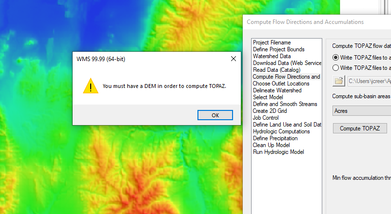
Missing DEM

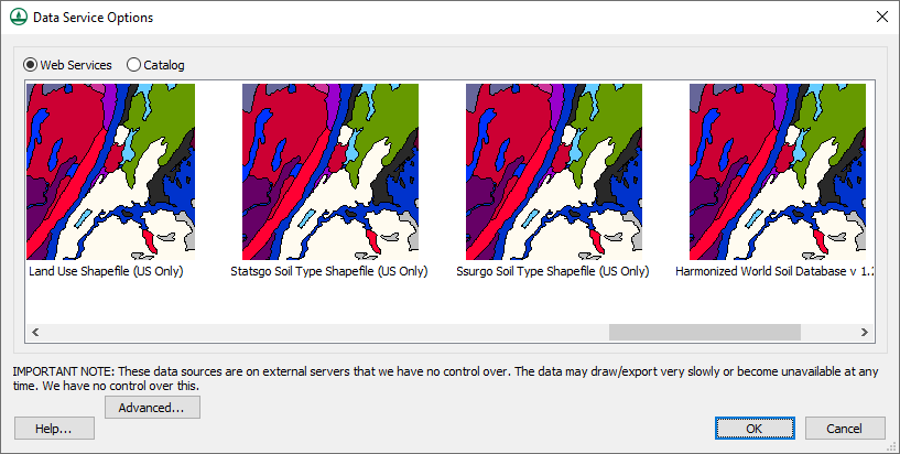
DEM data is required to run TOPAZ or TauDEM. A DEM can be imported from a file or downloaded from a web service. If you get an error stating that no DEM exists after you have imported the DEM data, this is typically because the DEM was not imported correctly.

TOPAZ unable to find DEM

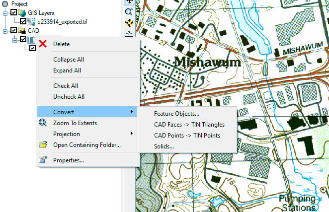
Often, the DEM has been imported as a raster file and is in the GIS data module. In order for TOPAZ or TauDEM to use this as a DEM it will need to be converted from a raster to a DEM using the Convert to | DEM right-click command in the GIS module.

Not Enough Data

In order for TOPAZ or TauDEM to work properly, a DEM is needed that has enough data to work with. When working on modeling very small areas, TOPAZ or TauDEM may fail to execute correctly because there is not enough data available to complete the process.

In order to fix this issue, it is recommended that you slightly expand the size of the area you are modeling. In particular, the resolution of the DEM being used may need to be increased. Use your best judgement as to how much additional data to add.

Too Much Data

The opposite of having too little data would be to have too much data which causes TOPAZ or TauDEM to slow down or stop running altogether. This typically happens when attempting to model a very large watershed. In this case, the issue typically isn’t related to problems with TOPAZ or TauDEM but is more likely related to the available processing power of the computer being used.

With many projects that have too much data, often much of that data is unnecessary. Often a lower resolution DEM can be used. When modeling a large watershed area, you should use your engineering judgement to find areas of greatest interest and then focus on those areas. If that is not possible, then you will need to find a way to increase your computer's processing power.

TOPAZ and TauDEM tools for delineating a basin. Try them out in WMS today!

Blog tags: 

Announcing SMS13.1 Beta

Aquaveo is pleased to announce the release of SMS 13.1 Beta! A number of new features have been added to this version, and we'd like to highlight a few of them.

3D Bridge

The new 3D Bridge feature allows creating a visual representation of a 3 bridge. This representation uses a 3D UGrid to visualize the bridge in the graphics window. After creating a 3D bridge, the feature can be visualized in an observation profile plot.Using the 3D feature allows generating a ceiling elevation dataset to represent the maximum water surface that can be reached at each point in the mesh at the intere. The bridge data can be exported as an XMUGRID file for use in multiple projects.

3D bridge example in SMS
Universal Select Tool

The Select Objects tool allows selecting multiple types of feature objects at the same time from the same tool. The selection information at the bottom of the screen changes if multiple types of objects are selected to show how many of each object is selected. The right-click menu changes to match the selected object type. If multiple feature object types are selected, then the right-click menus will be combined.

Extract Features

The Extract Features tool allows you to use a raster to generate feature arcs for channel centerlines, ridge centerlines, or channel cross sections and banklines. This can speed up the creation of the centerlines and cross sections by removing the need to manually create each feature individually. Options for this feature include the ability to extract all centerlines, extract all centerlines with one or more selected depression points, extracting a single centerline, or extracting channel banklines and cross sections.

Example of extracted feature arcs
HEC-RAS 1D

SMS 13.1 Beta includes support for creating and editing HEC-RAS 1D cross sections and attributes. These cross sections can be imported from HEC-RAS as SDF files and saved as a HEC-GeoRAS file for inclusion into a HEC-RAS project.

These are just a few of the new features in the SMS 13.1 beta. Try out these features and more by downloading the SMS 13.1 Beta today!

Blog tags: 

Using MODFLOW-NWT for Mine Dewatering

Have you tried dewatering a mine model using MODFLOW-NWT? MODFLOW-NWT is a version of MODFLOW provided by the USGS that uses a method to solve MODFLOW models that are non-linear due to unconfined cells or non-linear boundary conditions, creating an asymmetric results matrix. Because mines that need to be dewatered sit below the water table, cells within the simulation will become dry at times due to the removal of the water from the mine. MODFLOW-NWT is great for such situations as it handles dry cells well.

Modeled mine example

Mine dewatering models are often used when estimating the required flow capacity for the pumps used in the field. You can create a regional model to establish a baseline, then create one or more models with various pit depths to establish the best approach for the mine in question. While elevations cannot be set to transition during a MODFLOW run, multiple conceptual models can be created within the same project in order to keep all of the data together.

It’s important to remember the difference between wells and drains when creating the dewatering model. Drains only subtract water when the head is above the elevation of the drain. Therefore, drains can be used to represent the seepage face around the edges of the pit, and the drain elevations should be set to equal the ground surface elevations. The amount of water removed by a drain is related to the conductance of the material of the seepage face. Drains are generally used at the bottom and side seepage faces of the mine.

Wells remove a specific amount of flow, and can therefore dewater the cell they are in prior to dewatering the rest of the mine. MODFLOW-NWT, as mentioned previously, handles these dry cells very well, keeping them active in case they become wet again.

Because MODFLOW-NWT uses 3D grids, you should make sure the cells inside the pits are inactive. You do this by creating the boundary polygon, and then removing a "donut hole" of cells within the pit area. Use the Activate Cell(s) in Coverages tool to inactivate the cells. You’ll have to do this for each layer, and each layer should be on its own coverage.

Finally, always use the Model Check to make sure there aren't any obvious errors or missing values in any of the inputs. After MODFLOW-NWT finishes running, you should review the water table by looking at the drawdown output contours. You can also do this by switching to Ortho view and reviewing the head in the appropriate rows or columns.

Try out making a mine dewatering model using MODFLOW-NWT in GMS today!

Blog tags: 

Using Plots in CityWater

Any presentation about water distribution management can be improved with the right plots. CityWater has a number of different plots accessible through the plot icon on the Map View page that can be used by you to visualize the information available in each of your projects. These plots can be used in reports or presentations to help others understand details and specific time-based information you need to share.

The Plot icon on the Map view is a dynamic tool. If no nodes or links are selected, it will display a System Flow Balance plot when clicked. This plot shows the flow produced, consumed, and stored within your pipe network. You can select any point along each of the plot lines to see specific for that time.

CityWater System Flow Balance Flow

If you have a specific link or node selected (or more than one of either nodes or links selected), you can use the Layers tab drop-downs to select what will appear on the plot. This gives you a large number of possibilities for how the plot will appear. Some combinations do not have a plot available, and these will instead show the default System Flow Balance plot. We recommend taking the time to play around with the options to find the ones that will work best for you.

For example, the image below shows a plot with Demand, Links, and Minimum selected from the Node Layer, Link Layer, and Time drop-downs (respectively). As before, you can select any point along the plots to see specific details for the desired node or link.

CityWater Demand Plot

CityWater contains many other tools to help you visualize water flow and usage in your water distribution network all in an accessible and a convenient to use web environment. Learn more about how CityWater can help your organization today!

Blog tags: 

How SRH-2D and HY-8 Work Together

SMS allows using HY-8 to create culverts in SRH-2D models. HY-8 was created to model culvert profiles. When SRH-2D was being developed, structure boundary conditions were allowed to be linked HY-8 culverts to SRH-2D. Doing this permits SMS to make use of the more robust tools of HY-8 when designing culverts.

When designing a culvert for an SRH-2D model in SMS 13.0:

  1. Right-click on the SRH-2D BC coverage and open the HY-8 Options dialog.
  2. From the dialog, create the HY-8 file for the project.
  3. On the SRH-2D BC coverage, create two arcs for the culvert: one for the inlet side of the culvert and one for the outlet side.
  4. Select both arcs and open the SRH-2D Linear BC dialog.
  5. In the dialog, select the Culvert HY-8 option and launch HY-8 to connect the HY-8 file.
  6. In HY-8 design your culvert.
HY-8 with SRH-2D

There are a few items to keep in mind when creating your culvert:

  • Pay attention to where the culvert is located and how it snaps to the mesh in SMS. Designing your culvert for a location that doesn’t match up with your culvert is designed in HY-8 can cause discrepancies. Also, it helps to have the inflow entering the culvert at as close to a 90 degree angle as possible.
  • Note that the crest length for constant elevation roadway profiles is the length between embankments.
  • After the initial model run, the inflow values to the culvert may need to be adjusted and calibrated. If SRH-2D is showing lower or higher flow values, adjust the values in HY-8 as needed.
  • Using a monitor line at the inlet or outlet side of the culvert. The results of the monitor lines may be different than what HY-8 reports. Use this difference to calibrate the model.
  • 2D mesh elements are disabled between the culvert arcs during the model run.

HY-8 makes a great addition to SRH-2D in SMS. HY-8 is shipped with SMS, so feel free to try it out with your models today!

Blog tags: 

Using CAD data in GMS

Do you need to work with CAD data in your GMS project? This blog post will go over some of the ways to import, export, and convert CAD data in GMS.

Importing CAD Data

CAD data is common with project designs and is often necessary in order to import a CAD data file into GMS for an accurate view of the project. This is how CAD data can be imported:

  1. Select File | Open.
  2. In the Open dialog, it may help to change the File of Type field to specify a CAD format, such as "DWG/DXF".
  3. Navigate to the CAD file you wish to import and open the file.

CAD data can also be imported using the Open macro or using the drag-and-drop method like you would with any other file.

How to Convert CAD Data

For some projects, it is necessary to convert CAD data to another data type. You may also need to convert your project data into a CAD file format.

Converting from CAD

Converting options within GMS include the ability to convert CAD data to feature objects, TINs, and/or solids. This is done by right-clicking on the CAD object in the Project Explorer and selecting a command option in the Convert submenu.

CAD Data Conversion Menu in GMS

After selecting any of the conversion options, a dialog will be opened for more specifics on the conversion process.

Converting to CAD

GMS data can also be converted into CAD data by doing the following:

  1. In the Project Explorer and Graphics Window, hide any data you don’t want converted.
  2. Right-click in an empty spot in the Project Explorer and select the Convert to CAD command to bring up the Save CAD data dialog.
  3. Select location and name for your CAD file.

The CAD data that is converted from GMS will be saved as a DWG file or DXF file depending on what you select.

Exporting CAD Data

GMS also allows you to export CAD data in a project by doing the following:

  1. Right-click the CAD folder in the Project Explorer.
  2. Select Export to bring up the DWG/DXF Filename dialog.
  3. The options will appear to either select the DWG or the DXF file types to save as CAD data.

To find exported data, browse the project file folder. Another thing to note is that objects found within GMS must first be converted to CAD Data before being exported as CAD data.

Try importing, exporting, and converting CAD files in GMS today!

Blog tags: 

Importing Land Use and Soil Type into WMS

Have you needed to obtain land use or soil type data for your WMS project? Land use, or land cover, data is used to define the land use or cover of areas in the watershed such as urban, forested, farm, etc. Soil type data is typically used to control the movement of water in a watershed model. Data for land use or soil type can be added to your watershed project in WMS by using files on your computer or by downloading the data from a database.

Import a File

Files containing land use or soil type data are often contained in a shapefile, though other formats are possible. This file can be imported from your computer using the File | Open command. Once imported, the shapefile will appear in the GIS Module. It will likely need to be converted to the map coverage before being used in your watershed model.

Import From Web

Land use or soil type data can be obtained from online web services. To access these services, do the following:

  1. Select File | Add Data | Get Data from Map.
  2. In the Virtual Earth Map Locator, select the location of your project. If your project already has a set projection, then the location of your project should already be visible.
  3. In the Data Service Options dialog, select one of the web services containing land use or soil type data such as the Land Use Shapefile, Statsgo Soil Type Shapefile, or Harmonized World Soil Database.
  4. Save the land use or soil type data to your computer. The data will automatically be imported into your project as a shapefile in the GIS Module.
Data Service Options dialog showing land use and soil type options
Moving Land Use and Soil Type Data

In most cases, having land use or soil type data on a shapefile will not include the data in your watershed model. Most often the data will need to be moved from the shapefile to the Map module. To do this:

  1. Create a map coverage with the Land Use or Soil Type property. Land use data should be placed on a land use coverage and soil type data should be placed on a soil type coverage. Data may be lost if the wrong coverage type is used.
  2. After creating the correct map coverage, select the land use or soil type shapefile in the GIS module then select the Mapping | Shape to Feature Object command.
  3. When using the GIS to Feature Objects Wizard, select correct map coverage and make certain all of the attributes are correctly assigned.

Once you have imported land use or soil type data and it has been correctly converted to the Map module, it is ready to be used in your watershed model. Try out using land use and soil type data in WMS today!

Blog tags: 

Observation Arcs vs. SRH-2D Monitoring Lines

Have you ever wondered what is the difference between using an observation arc and using an SRH-2D monitoring line? Both make use of arcs drawn on map coverages and both are used to show the results of a model run. While they serve a similar purpose, there are significant differences between the two. This article will discuss some of these differences.

Observation Arcs

Observation arcs are made on an observation map coverage. This generic coverage can be used with nearly every numeric model in SMS. It is not specific to only SRH-2D. Observation arcs can be used to generate a profile plot based on the model run results. SMS does this by interpolating the results to locations along the observation arc.

An observation arc can be created before or after the model run. The arc can also be adjusted after the model run to change what is shown in an observation plot.

SRH-2D Monitoring Lines

SRH-2D monitoring lines are created on an SRH-2D monitor coverage. This is an SRH-2D specific coverage that will only work with an SRH-2D simulation. The monitor coverage must be included in the SRH-2D simulation during the simulation run in order for the monitoring lines to produce results. A plot from the monitor line can be viewed in the Simulation Run Queue during the model run.

When creating monitoring lines, arcs are drawn on the SRH-2D monitor coverage. It is important to pay attention to how these arcs snap to the SRH-2D mesh. Monitoring lines will follow the nodes of the mesh instead of interpolating to the location of the arc. For SRH-2D, this makes the results of the monitoring lines more accurate than observation arcs.

SHR-2D monitor lines snappingto mesh nodes

The results from the monitoring lines are found in the the *.dat file that starts with “LN”. If a change is made to a monitoring line after the simulation run, the simulation will need to be saved and run again to get the new results for the monitoring line.

Using both monitoring lines and observation arcs is common for many projects. Keeping in mind the differences will help you make better use of both of them. Try using observation arcs and monitoring lines in SMS today!

Blog tags: 

Tips for MODFLOW 6 in GMS 10.5 Beta

Have you had a chance to use MODFLOW 6 in the GMS 10.5 Beta? If you have, you may have noticed that MODFLOW 6 operates a little differently than other versions of MODFLOW. This is to allow for some additional tools and options.

When using MODFLOW 6 in GMS 10.5 Beta, here are a couple tricks to try out.

Having Multiple MODFLOW 6 Simulations in the Same Project

You can create multiple simulations in the same project by using the simulation workflow in GMS 10.5 beta. This is particularly useful when attempting to calibrate your project. The way this is done is by doing the following:

  1. Right-click on the simulation in the Project Explorer and select the Duplicate command. This will create a duplicate of the simulation that includes all the same parameters and uses the same grid.
  2. On the new simulation, change the parameter that needs to be calibrated, such as the head values or the pump values of the wells. It is generally best to only focus on one parameter change when calibrating the model.
  3. Run the new simulation and compare the results between the different simulations.
  4. Repeat this process with additional simulations to calibrate the model.
Duplicate command in the simulation menu
Running Multiple Simulations at the Same Time

After you have created multiple MODFLOW 6 simulations, you can run all of the simulations at once. This is done by doing the following:

  1. Right-click on the simulation folder and select the Save All and Run command.

The Simulation Run Queue dialog will display all of the simulation model runs. While the simulations are running, the Simulation Run Queue can be moved aside or minimized to allow you to keep using GMS. The results can be loaded into the project for you to review when the simulations have finished.

Sae All and Run command in the simulation folder menu

Additional features for MODFLOW 6 are still being added to GMS and will appear in future versions of the software. For now, check out MODFLOW 6 in GMS 10.5 beta today!

Blog tags: 

Sharing WMS Project Files

After completing your project in WMS, are you needing to share your project files with a client or colleague? When doing this, it is important that you send them all of the files related to the project. All of the files for the project should be shared in the same folder. This article will go over some of the important files to include.

The most important file to share is the WMS XMDF Project File (*.wms). This file contains many elements of your project, but also acts as a directory for the other files being used by your project. To improve application performance, the WMS project file does not contain all of the data necessary to open the project, so it is important to include all relevant files when sharing your project.

In addition to the WMS project file, it is important to include GIS files that are in the project. This would include any shapefiles, image files, raster files, or projection files. WMS will ask you to locate these files if they are not in the same directory as the WMS project file when the project is opened. If the GIS files are no longer relevant to the project, they should be removed from the project before saving and sharing the WMS project file.

GIS items in a WMS project

Another file that is important to include is the map file (*.map). This file contains all data related to feature objects and map coverages in the project. Without it, many projects may be unable to open. Similarly, the tree file (*.tre) is necessary to import hydraulic and hydrologic data. Grid (*.grd) are needed to import grid geometry.

When a model run has been completed, it is important for the solution (*.sol) and output (*.out) files to be included with the project file. Without these, whoever receives the files will be unable to see the results of your model run.

Finally, be certain to include model specific files, such as those for HEC-HMS or GSSHA. Refer to the model documentation for information on these files.

One trick to help include all files in your project, is to use the Save As command and save the project to a new folder. Then make certain to move that folder to a new directory and open the project file to see if any files are missing.

Now that you know a little more about WMS files, try sharing your WMS projects today!

Blog tags: 

Pages