Aquaveo & Water Resources Engineering News

How to Generate a Flood Depth Raster
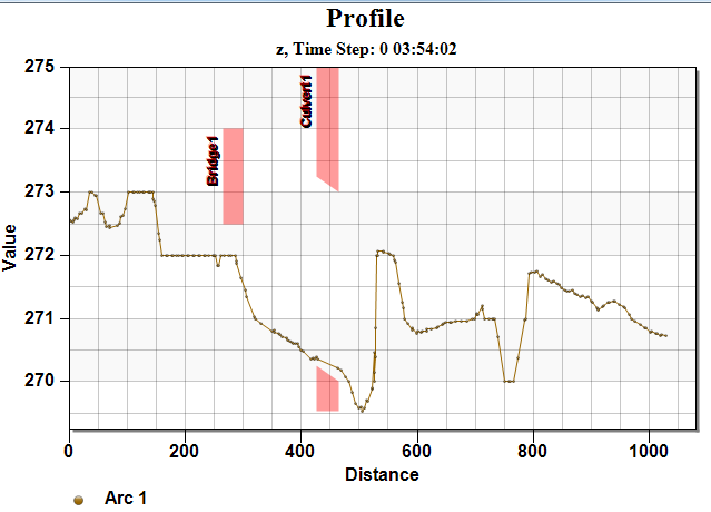
After running your model, such as SRH-2D, you will have a water surface elevation (WSE) dataset. Did you know that, starting in SMS 13.0, you can use the WSE dataset to create a raster showing the flood depths?

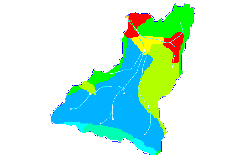
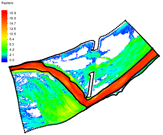
SMS can create a flood depth raster by using the WSE solution dataset at a specific time step and comparing it to the initial elevation data. Using both of these datasets, it can then generate a raster that shows the flooded areas for a specific time step.

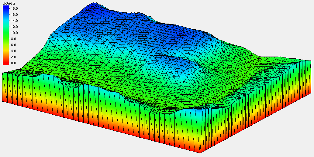
In order to create a flood depth raster your project will need a WSE solution dataset and an elevation raster. Once you have a raster:

  1. Select the desired time step for your WSE solution dataset.
  2. Right-click on the raster and select Convert To | Flood Depths.
  3. In the Select Geometry and Dataset dialog, select a geometry containing your WSE solution dataset. The selected geometry can be either a 2D mesh or a 2D scatter set.
  4. Next select the WSE solution dataset.
  5. Click OK to close the Select Geometry and Dataset dialog, which will launch the Save As dialog.
  6. Creating a name for your raster and click Save. (Note that the file should be saved as a "GeoTIFF Files (*.tif)".
  7. Hide the mesh and elevation raster to be able to view your new flood depth raster.

It should be noted that it may take a few minutes for the flood depth raster to be generated depending on the available processing power of your machine. Since a raster file is saved during the process, the file is available for use in other applications if desired. Coordinate data is saved with the file.

Now that you know to create flood depth rasters, try using them in your SRH-2D projects in SMS.

Blog tags: 

Changing an Existing Model to be a Predictive Model

When you have a completed GMS model, you can use that same model to create a predictive model. A predictive model is used to make predictions based on hypothetical future scenarios. For example, you may need to create a model that predicts if an aquifer will experience strain with an increased population drawing from the aquifer in the model area.

Groundwater model

In general, a predictive model is created by using an existing model, then altering an aspect of that model based on the hypothesis. You then run the model again and compare your results with your prediction. Any version of MODFLOW, or any of the other available numeric models in GMS, can be used to create a predictive model.

One method of setting up a predictive model might be as follows:

  1. Create and run a steady state model
  2. Calibrate the model to reduce error in the predictive model
  3. Set the transient settings to a future date
  4. Run the transient model

It is important for you to have an expectation of the outcome of the model run so that you can compare the results with that expectation. When the model run is completed, carefully review the model run results to determine the accuracy of the predictions. When creating a predictive model, you can make use of stochastic analyses.

If the predictive model seems to be far outside of your expectations, then you will need to troubleshoot the existing model before running the predictive model. Using a poorly developed existing model often leads to issues in the predictive model. Make certain the existing model has been well calibrated to closely match the field-observed values. If possible, calibrate the existing model to multiple sets of observation data before creating a predictive model.

Now that you know some of the principles in developing a predictive model, creating your own predictive model in GMS today!

Blog tags: 

Tips for Managing Cross Sections in WMS

Cross sections are commonly used in 1D models within WMS. Here we discuss a few things to help you better model using cross sections.

When you create cross sections in WMS, you must create them on "1D-Hyd Cross Section" coverage. You then create the arcs on this coverage to represent the cross sections.There are a few things you should remember when setting up your cross sections:

  • Cross sections should be located at fairly frequent intervals along the river. This makes sure the characterization of the stream channel and floodplain flow and capacity is accurate, which gives you better results.
  • You should place cross sections especially at locations of significant change, where levees begin and end, at hydraulic structures, and around stream junctions.
  • The cross section arcs should generally stretch from one side of the river floodplain to the other.
  • They should be generally perpendicular to the river arc where they cross.
  • Cross section arcs should not cross each other.
Hydraulic Model Example with Cross Sections

In addition to the above, each cross section should have the following required information:

  • River name
  • Reach name
  • River station
  • Description
  • Station–elevation data
  • Downstream reach lengths
  • Manning’s n values
  • Main channel bank stations
  • Contraction and expansion coefficients

It is recommended that the station number be visible on the map view to make the cross sections more identifiable. This can be enabled in the Display Options dialog. When numbering stations, they must be in ascending numerical order from downstream to upstream. If changes are made, be sure to renumber the stations.

Converting an arc into a cross section arc can be done automatically or manually. You can automatically do it by taking the following steps:

  1. Define or import a TIN.
  2. Create an area property coverage, a centerline coverage, and a 1D-Hyd cross section coverage.
  3. Use the Extract Cross Section command to extrude the cross sections from the 2D arcs.

To manually create a cross section arc:

  1. Double-click on the cross section arc and select Assign Cross Section.
  2. Define the various elevations and data as desired.

Try out these tips and procedures today in the WMS Community Edition!

Blog tags: 

Using Internal Sinks and Links in SRH-2D

Do you have an SRH-2D project that requires placing a drain inside the mesh? Or perhaps you have two seperate meshes in your project where you need to have water flowing between them? Both of these scenarios can be resolved by respectively using the internal sink and link boundary conditions.

Internal Sink Boundary Condition

The internal sink boundary condition is assigned to an arc on an SRH-2D boundary condition map coverage. Unlike an inflow or outflow boundary condition, an internal sink is assigned to an arc that is inside the mesh boundaries.

An internal sink can simulate wells, drains or other points of outflow. It can also simulate a source by specifying a negative number for the flow.

It should be noted that an internal sink boundary condition should not be used as a model’s primary source of inflow or outflow. Inflow and outflow boundary conditions should be placed on the mesh boundary.

Links

Link boundary conditions can be used to simulate moving water between two different meshes or two different areas of the same mesh. Links can sometimes be used to make a simple representation of a pipe or similar structure connecting two areas.

Links are made by making two arcs on an SRH-2D boundary condition coverage. Both arcs are selected when assigning the Link property type. One arc should be assigned as the link inflow boundary condition and the other arcs should be assigned as the link outflow.

Example of an link boundary conditions

It should be noted that link boundary conditions should not be used to model culverts or other such structures. Also, link boundary conditions should not be used as the primary inflow or outflow source for a project.

Now that you know a little more about using internal sink and link boundary conditions, try using them in your SRH-2D projects in SMS.

Blog tags: 

Using MODFLOW Native Files

If you have been using MODFLOW with GMS for any amount of time, you have likely noticed that GMS uses a modified version of the MODFLOW files. This is so that the MODFLOW files can be used more efficiently by the GMS interface.

However, there are times when a project may require using the native MODFLOW files. This is often necessary when opening a MODFLOW project that was not originally created in GMS, or when sharing a project with someone who does not have access to GMS.

When importing native MODFLOW files into GMS, there are some important concepts to keep in mind:

  • You will need to start by importing either the NAM file or MFN file. These files contain a directory for the other files in the MODFLOW project and how they should be opened.
  • It is important to keep all of the MODFLOW files together in the same directory. Having only the NAME or MFN file will not be enough to open the MODLOW project.
  • Files for the packages used with the project will typically have a file extension that matches the package. For example, the Wells package will have the extension "*.wel".
  • All native MODFLOW files can be opened and reviewed using a text editor if needed. See the MODFLOW user guide for information on the file format.
The Save Native Text Copy option

Native MODFLOW files can be exported from GMS by turning on the Save Native Text Copy option in the MODFLOW Global/Basic Package dialog. When exporting native MODFLOW files, keep the following in mind:

  • GMS will create a separate directory with the native MODFLOW files. This directory will typically be the project name with "_text" appended to it. For example, if the project is named "Aquifer", the directory will be named "Aquifer_text".
  • All files in this directory should be kept together.
  • As mentioned before, the files can be reviewed using a text editor.

With GMS 10.4, MODFLOW 6 native files can be imported and exported.

Being able to use native MODFLOW files can greatly enhance collaboration with projects. Try out importing and exporting native MODFLOW files in GMS today!

Blog tags: 

Obtaining Nonstandard Data for Curve Numbers

Calculating curve numbers is a necessary process for many WMS projects. WMS contains a number of tables with suggested soil and land use data for use in calculating the curve number. These are not comprehensive lists of every possible soil data resource, however. These are, only those that are readily downloadable through WMS.

So what do you do if you need to use soil or land use data from a location without data readily available in WMS? You can use nonstandard soil or land use data by creating a file with the data formatted as a table. The format of those land table files can be applied to create a table for any soil data source, such as local shapefiles developed for specific projects.

Example of a land use shapefile

The format for these files is a set of columns as follows:

  1. Soil ID number
  2. Category Label
  3. Hydrologic soil group A
  4. Hydrologic soil group B
  5. Hydrologic soil group C
  6. Hydrologic soil group D

Once you have created a text file with your soil or land use data, import it into WMS as you would any other soil or land use data.

If you’re building your own table for your soil data, there are sources for the tables and charts to help facilitate estimating the curve numbers to put into the table.

For an explanation of or introduction to SCS or runoff curve numbers, a good source is the National Conservation District Employees Association. Their guidance may help clarify the process of creating your own curve numbers.

Additional sources can also be found for soil or land use data. Use whichever data source you feel is appropriate for your project. As long as the data is formatted correctly, WMS should be able to import it.

Try out importing soil and land use data from locations around the world using WMS today!

Blog tags: 

Using STL Files in SMS

Starting in SMS 13.0, SMS can now make use of STL files.

STL files use tessellation, the process of mimicking a surface by assigning surface coordinates to a repeated pattern of polygons. In the case of STL files, triangles are used to make a 3D mesh that can effectively be rendered into any shape needed including landscapes.

STL files are typically used for 3D printing. They also can be used for the modeling landscapes. There are several methods for creating these files. This post will not attempt to cover the specifics of those methods as other places cover how do this.

Uploading and Using STL Files

In SMS, STL files are used to model terrain. Once you have created an STL file, importing it by using the File | Open command or dragging-and-dropping the file into SMS.

When uploaded, the file is automatically transformed into a Ugrid and adjusted for the associated z values. This UGrid can then be used for all the normal uses of such in SMS.

Example of an STL file loaded into SMS

It is important to mention that the z values may or may not be representative of the elevation depending on the source of the STL file used. Fortunately, there is a way to handle such cases in SMS. After import, the Ugrid can be converted into a 2D scatter dataset. The scatter can then be interpolated to a mesh or modified with the data calculator. If desired, tim and dim files representing that data can then be created as usual.

Exporting STL Files

To create an STL file, you must have a UGrid with the corresponding elevation data attached. This UGrid must consist of only triangular elements.

Export the STL file by:

  1. Right-click on the UGrid and select the Export command.
  2. Then select a (*.stl) file type before saving the file.

There are two STL file type available for export. The binary option is often used since it requires less memory. The ASCII file is more user friendly if the file needs to be inspected. Both save data by recording the coordinates of the vertices associated with each triangle. If unaccompanied by other files, the Ugrid will also have to be manually associated with the correct projection after uploading.

We hope to add more functionality for STL files in the future. Try using STL files with your SMS projects today!

Blog tags: 

Exploring MODFLOW Head Boundary Packages

GMS allows using a number of different MODFLOW head boundary packages (GHB, RIV, STR, SFR, etc.) to indicate flow in or out of your model. These packages often appear to be similar. To the differences between them, here we discuss a few of these packages.

Example of MODFLOW head boundary packages available in GMS
General Head

The General Head Boundary (GHB) is, conceptually, a fixed head far from the model where it is assumed to be a fixed head with time (i.e., the river or head will not be affected by the model stresses over time). The purpose of using this boundary condition is to avoid unnecessarily extending the model domain outward to meet the element influencing the head in the model. As a result, the general head condition is usually assigned along the outside edge of the model domain.

General head cells are often used to simulate lakes. General head conditions are specified by assigning a head and a conductance to a selected set of cells. If the water table elevation rises above the specified head, water flows out of the aquifer. If the water table elevation falls below the specified head, water flows into the aquifer. In both cases, the flow rate is proportional to the head difference, and the constant of proportionality is the conductance.

River

The MODFLOW River (RIV) package only tracks flow between the aquifer and the river. With the River Package, once water has entered the river, it is lost to the model.

Stream

Unlike the River package, the Stream (STR) package routes flow through the stream. The water can travel downstream and possibly re-enter the aquifer at another point. The Stream package also allow periodic drying. However, there are more restrictions than in the River package.

Also unlike the River package, the Stream package calculates the water depth based on the flow rather than it being manually entered. There are several different options available for calculating water depth, including using Manning’s equation or a depth versus flow table.

The Stream package divides streams into reaches and segments. It models effects of rivers on aquifers while tracking flow in river. Interaction between surficial streams and the groundwater for the Stream package uses Manning’s equation and simple channel hydraulics to compute the stage in the stream.

Streamflow Routing

This Streamflow Routing (SFR2) package is similar to the Stream package. Though it has more restrictions than STR, it has more sophisticated hydraulics and routing options.

These are just the most commonly-used of over a dozen different MODFLOW head boundary packages that can be used with GMS. Go ahead and explore the different MODFLOW packages available in GMS today!

Blog tags: 

Downloading NLCD Data

One of the crucial elements of any project is having data. WMS makes use of a large number of data sources. One type of data that we find frequently used is National Land Cover Database (NLCD) data. NLCD is provided by the MRLC (Multi-Resolution Land Characteristics Consortium) as a large collection of raster datasets.

Here are three ways this data can be imported into WMS.

Direct Download

NLCD data can be downloaded from the MRLC site. Much of the other data available on the MRLC site can also be used with WMS.

Downloaded NLCD data can be opened in WMS by selecting the Open macro, browsing to the folder containing the downloaded data, and selecting the desired raster. WMS should be able to recognize the data file and bring it into your project.

Using the Modeling Wizard

NLCD data can also be downloaded while using the Hydrologic Modeling Wizard or the HY-8 Modeling Wizard. To do this:

  1. Start the Hydrologic Modeling Wizard or the HY-8 Modeling Wizard
  2. Create the project in the first step
  3. Define your project bounds and set the project projection
  4. In the Watershed Data step, turn on the Use web services option
  5. In the Download Data (Web Services) step, select one of the NLCD data types
  6. Click the Download Data From Web button to download and import your NLCD data
  7. Enter a raster cell size for the data
  8. Save the data as a file
Using the Get Data Tool

Downloading NLCD data can also be obtained by using the Get Data tool. To use this tool, your project must have a projection already defined. When you have a projection set, do the following:

  1. Using the Get Data tool, click-and-drag a box in the Graphics Window that covers the area where you want NLCD data
  2. Save a file with the NLCD data
  3. Enter the raster cell size for the data
Downloading NLCD data

You might also notice that a lot of other data sources are available through the Modeling Wizard and Get Data tool. Feel free to try downloading data from these sources for your WMS projects.

Blog tags: 

Using the Plot Data Coverage

Have you generated a plot in SMS and found it was difficult to see where a bridge, culvert, or other structure location matched up with the plot? The Plot Data coverage helps make them more visible, making an observation coverage more meaningful in a profile plot.

Typically, a profile shows some desired value such as water surface elevation or the riverbed elevation. This data can be more useful in many cases if structures are displayed on the plot as well. A Plot Data coverage allows creating polygons over structures that then helps display the location of the structure on the plot profile.

To use the Plot Data coverage, do the following:

  1. In the Map Module, create a new coverage with the Plot Data type.
  2. In this new Plot Data coverage, create a polygon over the area of interest.
  3. Double-click on the Polygon to assign attributes in the Plot Data dialog.
  4. Create an observation arc that includes the area of interest.
  5. Create an observation profile plot.
  6. In the Plot Data Options, turn on the Plot Data coverage.

The profile plot will now show where the polygon on the Plot Data coverage aligns with the profile.

Example of a Plot Data coverage used in a plot profile

For example, if you want to consider the impact of a new bridge placement on the flow of a river, you could create a polygon representing the bridge location. When included in the profile, this could help you visualize placing a bridge at that location along the river and at the indicated height. If water elevation data is available, such as from an SRH 2D simulation, the height of the bridge can be easily compared with elevation profile of the water surface. This could be helpful in considering if the bridge would be washed out or flooded during periods of heavy rain when the river swells.

Culverts can similarly be shown on the profile by using the Plot Data coverage. Likewise, obstructions or structures of any shape could also be shown in the profile using the Plot Data coverage. Multiple plot data coverages could be used when there is a desire to layer structures such as a hypothetical bridge and the supporting abutments or columns.

Try out using the Plot Data coverage in SMS today!

Blog tags: 

Pages