Aquaveo & Water Resources Engineering News

Using Mass Flux Computations

Are you wanting to compute the mass flux for a group of MODFLOW boundary conditions? The mass flux is the rate of mass flow per unit area, or mass per time per area. Computing this can quantify the strength of contaminants at a particular location in your model.

Use the MT3DMS or MT3D-USGS model to compute the mass flux at specific location. To do this:

  1. First create and run a MODFLOW model.
  2. Then create an MT3DMS or MT3D-USGS simulation with all relevant parameters set and contaminant species defined.
  3. Make certain the Transportation Observation Package is turned on in the MT3DMS/RT3D Packages dialog.
  4. If it is not already in the model, create a conceptual model with the MT3DMS/MT3D-USGS defined species.
  5. Create a map coverage with the observation point option for the species turned on.
  6. Create points on the coverage at the locations where you want to to observe mass flux.
  7. Assign these points as observation points and enter attributes as needed.
  8. Access the Transport Observation Package dialog through the MT3DMS or MT3D-USGS menu.
  9. Turn on the Compute mass flux at source/sinks option.
  10. Run the model.

MT3MDS/MT3D-USGS will compute the mass flux at each observation point. The computation is done using the units set for the input concentration. Typically, these are the units used for the display projection in GMS. So if your project is using U.S. survey feet, then your mass flux will be calculated as ft^3*mg/L. If varying units are used in the concentrations, then conversions must be done before calculating the mass flux.

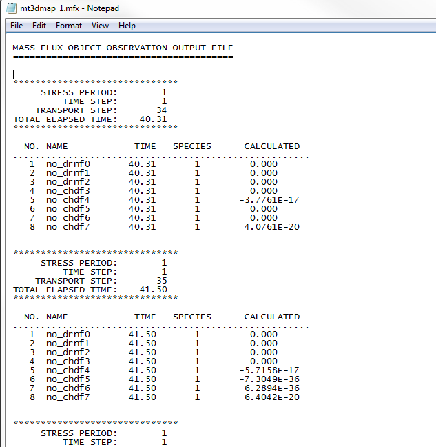
The mass flux will be contained in a dataset file with the “.mfx” file extension. This file can be opened using any text editor. The file will show the calculated mass flux for each time step and for each source or sink included in the model.

Hopefully, you now understand a little more about calculating mass flux in GMS. Try out mass flux calculations and other features in GMS today!

Blog tags: 

Visualizing Meteorological Data

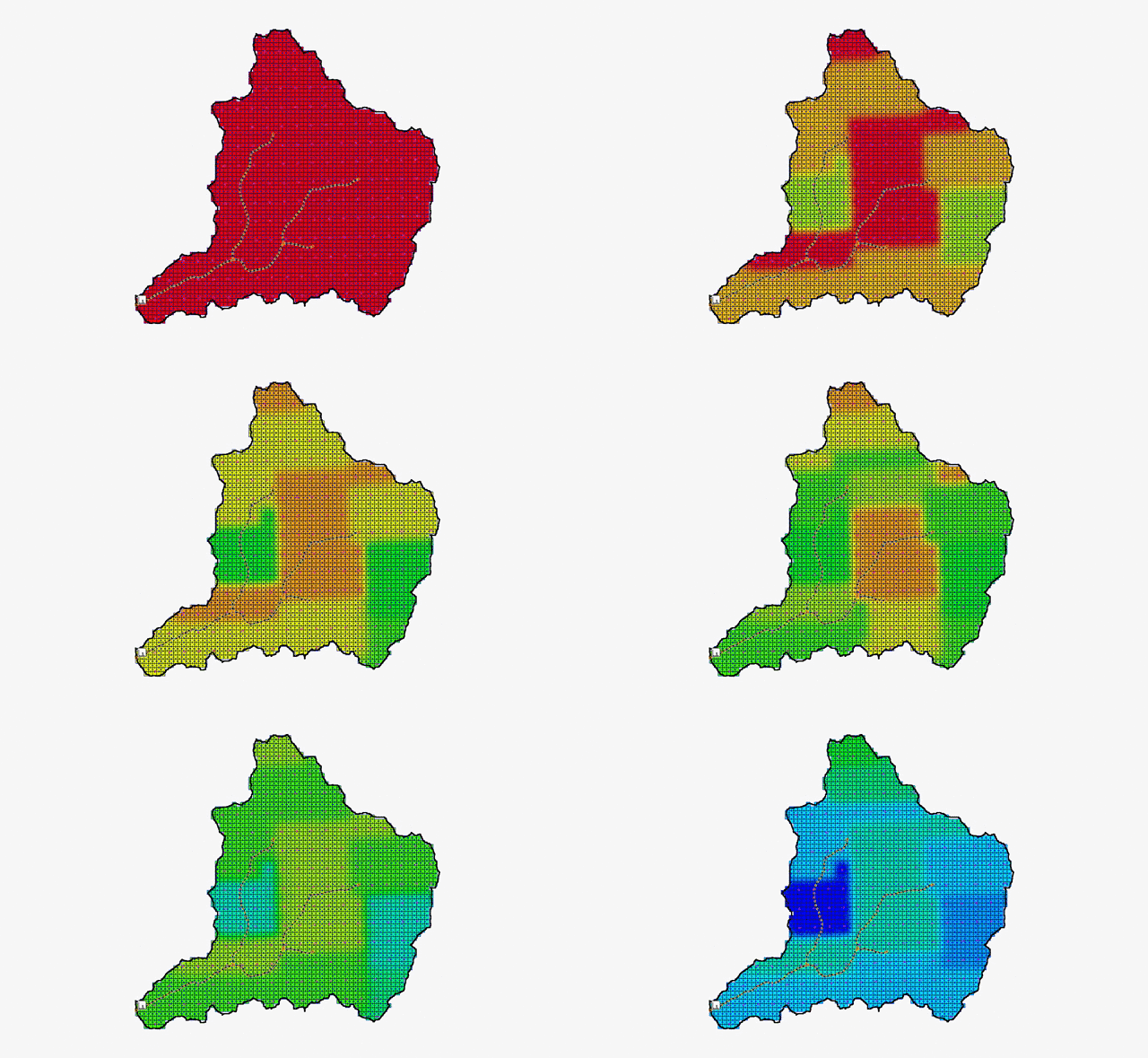
Do have rainfall data you would like to visualize in WMS? Inside WMS there are a couple tools to make your rainfall data visually interesting.

After you have imported your precipitation data, such as NEXRAD data, you can adjust your display options and/or create an animation.

Adjusting the Display Options

  1. Use the Display | Display Options command to open the Display Options dialog.
  2. Adjust your display options to show the data you want captured. It is recommended to turn on the Contours options.
  3. If using the Contours option, right-click on your rainfall dataset under 2D Grid Data and select Contour Options to open the Contour Options dialog.
  4. Adjust the contour method and interval to best display your rainfall data.
  5. With the down arrow key on the keyboard, step through the time steps in the properties window on the right sidebar to see how the precipitation varies.

Creating an Animation Loop

  1. Select your rainfall dataset in the 2-D Grid Module. The selected dataset will be used to create the film loop and can be cumulative or incremental. View incremental rainfall datasets in the same way as cumulative datasets.
  2. Select the Data | Film Loop command to open the Film Loop Setup Wizard. This wizard needs to be opened with the 2-D Grid Module active in order to have access to the meteorological data options.
  3. The first step in the Film Loop Setup wizard is essentially the same as creating any other animation through WMS. Select the location where the animation file will be saved and the type of film loop to generate.
  4. The second step of the Film Loop Setup wizard is to set the desired time step options for the rainfall data.
  5. The final step is where you will finalize the display options of the animation, and click Finish.
  6. WMS will take a few moments to create and save the animation file. The animation will start playing as soon as the saving process is complete.

When all is done, you can view your animation using the AVI play provided with the WMS installation, or you can use another application, such as GoogleEarth. The animation will display the movement of the storm through the selected time steps.

Try visualizing meteorological data in WMS today!

Blog tags: 

5 Ways to Make Projects Work Faster

Have you ever noticed your SMS project taking a long time to open or running slow when you’re working in it? Does the project seem to lag when zooming or panning? Perhaps it is time to clean up your project so it runs faster.

While not every project can be made to load or work faster, there are some items that can be done to speed things up. In general, a project that takes a long time to open or operates slowly is usually a larger project with many large components. Having a detailed mesh or large raster files will often slow down SMS on many machines.

To get things going faster, here are five tips for making your project work faster.

1. Change Display Options

Having more objects visible in the Graphics Window will impact how quickly SMS can operate. When SMS is trying to display a lot of data, it will slow down. By reducing the amount of visual information in the Graphics Window, SMS can process faster. This can be done in two ways.

The first method is to hide items in the Project Explorer, such as images or map coverages that are not being currently used. Having several images and rasters showing can particularly slow down a project.

The second method is to open the Display Options dialog and turn off options that are not needed. Contours and vector displays and displaying mesh elements can particularly slow down SMS. Keeping the total number of active display options to a minimum when working with large projects can speed things up for you.

Finally, when opening a large project or file, turning off all or nearly all of the display options can reduce the time it takes to open.

2. Remove Unnecessary Files

Does your project have a lot of data in it? There is a chance that this is slowing things down. Removing files that are no longer needed from the project can help.

If you have already interpolated your elevation data to your mesh or grid, then that data can be removed. If you have a dynamic image in your project, SMS will update the image every time you zoom or pan. Replacing the dynamic image with a static image and removing the dynamic image will speed things up. Shapefiles can also be removed from the project once you’ve interpolated or converted their data.

3. Resample Rasters

Having a large raster or lidar file is not really that unusual. However, having a 10 gigabyte (or larger) file loaded into your project will make SMS run slower. In many cases, all of the data contained in these large files isn’t necessary for the model to run and obtain accurate results.

Resampling the raster to a lower resolution can help. If the raster has already been loaded into SMS, right-click on the raster in the Project Explorer and select Export to resample it. When done resampling and adding the resampled image, remember to remove the original file from the project.

SMS uses a simple resample process. For more controlled application of rasters, other software can be used.

4. Refine the Mesh or Grid

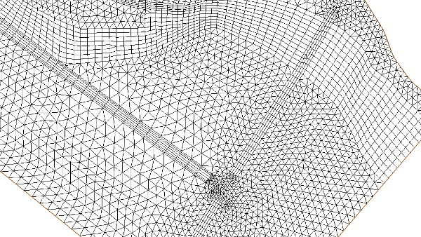
Are you working with a detailed mesh or grid with a lot of elements? While fine detailed meshes and grids are sometimes needed, only certain parts of the mesh or grid may need those details. The rest of the mesh or grid can have larger elements without affecting the accuracy of the project.

For example, when using a mesh for a riverine model, fine elements are generally only needed around the channel and structures. The mesh will often still be suitable using larger elements further away from these key areas.
5. Keep the Number of Simulations Small

Having a lot of simulations in one project file is tempting. For models that use the simulation process, such as SRH-2D, there is no limit to the number you can create.

However, for each simulation in your project file, SMS has to load that instance of the simulation. While all of your simulations may use the same geometry, items such as the model parameters will have been duplicated and increase the file size.

Therefore, when possible, it is best to limit the number of simulations in the project. You may want to create copies of your project then only include simulations in each project that share a particular variable. For example, one project file might have simulations with 10 year predictions while another project file has simulations with 100 year predictions.

Try out any of these tips with your SMS projects today!
Blog tags: 

5 Ways to Select Arcs in GMS

Everyone knows you can select an arc in GMS by using the Select Arcs tool and clicking on the desired arc. But did you know there are five different ways to select one or more arcs? Here’s a quick rundown of all of them:

  1. Use the Select Arcs tool to click on a single arc. This is the most common way to select an arc, but it only allows you to select one at a time. If you have multiple arcs you need selected, there are better, more efficient ways to select them.
  2. Use the Select Arcs tool while pressing the Shift or Ctrl key to select multiple specific arcs. This allows you to select only the desired arcs for whatever purpose you wish. This method includes all of the precision of the first method, but can take a long time if you have many different arcs to select. The next three methods allow you to more quickly select larger numbers of arcs.
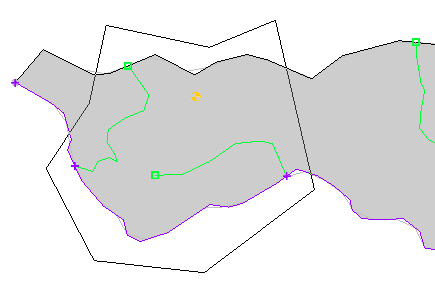
  3. Use the Select Arcs tool to drag a box around multiple arcs to select them. All arcs where both nodes of the arc are contained within the box wil be selected. Arcs where one node is outside of the box will not be selected. The click and drag method provides a quick method for selecting multiple arcs, but is not as accurate.
  4. Use the Select All command in the Edit menu to select all the arcs in the project. Just make sure to have the Select Arcs tool selected first so GMS knows what to select. The Unselect All command can be used to deselect everything when you’re done, if desired.
  5. The Select With Poly command in the Edit menu lets you draw out a polygon around the arcs you want selected. Keep in mind that both ends of an arc must be within the polygon in order for it to be selected.

Try out these options today in the GMS Community Edition.

Edit: This post was updated on 7/20/2018 to correct information in methods 2 and 3.
Blog tags: 

Using Software Graphics Mode

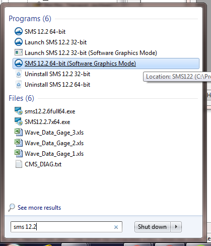
Have you ever noticed in your Start Menu that GMS, SMS, and WMS all have a version of the software executable that says "Software Graphics Mode"? Do you wonder what this is used for?

The software graphics mode was created to help resolve issues when there is a mismatch between the XMS software and the graphics card on a computer running the software. While we work to have XMS function on a wide range of graphics cards, some graphics cards do not support current versions of XMS.

When there is a mismatch, you might experience difficulty running the software. Issues we’ve seen happen include:

  • Having objects disappear from the Graphics Window when drawing new objects.
  • When changing views, objects in the Graphics Window disappear completely when they should still be visible.
  • Objects that appear in the Graphics Window that cannot be hidden or removed.
  • In some cases, the XMS application will not start.
  • In other cases, the XMS application will close suddenly.

Using the software graphics mode causes the machine running the XMS application to bypass the graphics card. Think of it as “safe mode” for XMS. Doing this places a heavier burden on the machine’s memory and processor, but it typically allows the XMS application to be used without the problems being caused by the graphics card.

To access the software graphics mode, go to your Start Menu and select the desired XMS executable with "Software Graphics Mode" in the title.

If using the software graphics mode resolves the issue you were experiencing, there is still one more thing to do: update your graphics card drivers.

Updating your graphics card drivers often resolve the issues being caused by the mismatch between the XMS application and the graphics card. Follow the standard procedure for updating the graphics card drivers for your operating system. In some cases, you will need to go to the graphic card manufacturer's website to update the drivers.

Once the graphic card drivers have been updated, you can usually continue to use the XMS application without using the software graphics mode.

And if updating the graphics card drivers doesn’t work, do not hesitate to contact Aquaveo Support for additional help.

Blog tags: 

Viewing Mesh Quality and ARR Plots

After generating a mesh in SMS, we hope the mesh has everything you need for a project and nothing else needs to be done for the mesh. While this is often the case, some meshes do not generate as nicely as we would like. There might be small areas where solution variables change rapidly or spots with too many connecting elements.

Quality issues in a mesh can cause issues with the model results, so you can save a lot of time by reviewing the mesh quality before running your simulation.

SMS provide a number of tools for evaluating the mesh quality. Two of these tools are the Mesh Quality Display Options and ARR Plots.

Mesh Quality Display Options

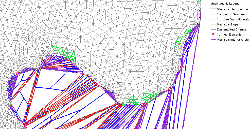
After you’ve generated your mesh, one of the fastest ways to see the quality of the mesh is to turn on the Mesh Quality Options in the Display Options menu. To do this:

  1. Open the Display Options dialog
  2. Go to the Mesh tab and turn on the Mesh Quality option
  3. Click the Options button to change how the various mesh quality checks are displayed

After turning on the mesh quality option, you will be able to more clearly see where there are potential quality issues. Each quality issues has its own color or symbol which is displayed in the legend. Looking over the mesh, it can become clear where there are potential issues.

ARR Plots

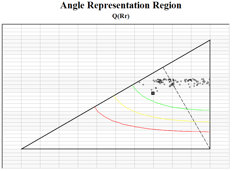
An Area Representation Region (ARR) plot can help you assess the overall quality of the mesh. To create an ARR plot:

  1. Select the mesh you want to review
  2. Open the Plot Wizard
  3. Select the ARR Mesh Quality option from the list on the left and click Finish

When the ARR Plot has been generated, you can use the plot to see the mesh quality.

The plot has a point for each element. Points above the green line are good elements. Points below the red line are elements that should be reviewed and fixed. Points between the green and red line are elements that should be reviewed to see if they should be fixed.

Clicking on a point in the ARR plot will highlight the corresponding element on the mesh in the Graphics Window.

Try these options out in the SMS today!

Blog tags: 

Using Contours to View Contaminant Flow into a Well

You’ve finished creating a model tracking the contaminant flow into a well. Your values look good and you’re certain the model executed successfully. The only problem is that when you look at you model, the visual representation of the contaminant flow is rather lackluster. You can tell there is flow towards the well, but it’s hard to clearly see how much of the contaminant is entering. Knowing this information can sometimes make a significant difference.

The solution to this dilemma is to adjust your contour options. In particular, two options will help you see the contaminant flow more clearly: adjusting the contour interval and adjusting the contour range.

Contour Intervals

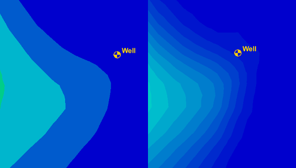
When looking at your contaminant flow, it might appear as though the contaminant has not reached your well. This can be misleading if looking at the model zoomed in and with a small contour interval. Smaller amounts of the contaminant might have reached the well, but we wouldn’t know because the interval is too small to show that level of detail.

After turning on contours for the solution set, increase the intervals around the well by doing the following.

  1. Zoom in on the well area.
  2. Make the contaminant dataset active in the Project Explorer.
  3. Click the Contour Options macro.
  4. In the Dataset Contour Options dialog, increase the contour interval value.

Now the contour has been broken up into more intervals, making it easier to see when the contaminant first reaches the well.

Contour Ranges

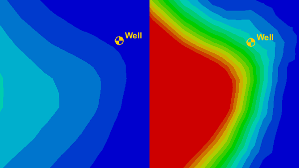
Another option is to change the contour range so it targets the values near the well. After turning on contours for the solution set, change the range by doing the following.

  1. Zoom in on the well area.
  2. Make the contaminant dataset active in the Project Explorer.
  3. Click the Contour Options macro.
  4. Turn on the Specify a range option.
  5. Enter minimum and maximum range values that focus on those contour values near the well.

Now the contours specifically highlight the contaminant flow into the well.

By experimenting with the different contour options, you can find the one that best shows contaminant flow in your project. Try this today in GMS!

Blog tags: 

3 Ways to Troubleshoot WMS Basin Issues

Have you noticed your model’s basin isn't what you hoped it to be? When you create a solid watershed model, there are a few common issues that can make the model not work as intended. These include:

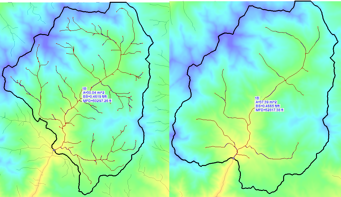
  1. Having a flow accumulation threshold that is too low or too high.
  2. Having one or more outlets in the wrong location for proper definition of the sub-basins and basins.
  3. Trying to work with a project area that is too large or too small for the intended purpose.

Flow Accumulation Threshold

Setting the correct flow accumulation threshold is very important. If you set the flow accumulation threshold too low, it may not accurately show the information you need, leaving sections of the watershed model reporting dry conditions. If you set it too high, you can be overwhelmed with too much information. It is good practice to try multiple levels to see which provides the most accurate results for the project. You can adjust this setting by doing the following:

  1. Open the Hydrological Modeling Wizard dialog.
  2. Select Compute Flow Directions and Accumulations (TOPAZ) from the list on the left.
  3. Enter the desired Min flow accumulation threshold and close the dialog.

Adjusting the Outlet

Placing an outlet in the wrong location causes the entire structure of the stream system to change dramatically. This can produce sub-basins quite different than desired, which can lead to results not lining up as expected. Remember that everything upstream from an outlet will be part of the same sub-basin or basin, so be careful when placing your outlets for each sub-basin as well as for the full basin.

Project Area

Sometimes, you may select a larger area than necessary for your model, or you may select an area too small for the project to produce useful results. If the area is too large, the desired details may not show up in your results. If the selected area is too small, you may not have enough data on which to base your decisions for the watershed.

If you keep these ideas in mind, your watersheds will better represent the areas you're modeling. Experiment with this today in the WMS Community Edition.

Blog tags: 

Stockholm GMS Training 2018

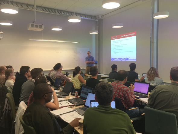
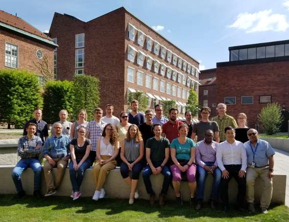
Aquaveo recently taught a three-day GMS training session hosted by the School of Engineering Science at the KTH Royal Institute of Technology in Stockholm, Sweden. The institute’s Prosun Bhattacharya arranged and coordinated the training session.

From May 15-18, 2018, Alan Lemon and Hoang Tran presented on a wide range of topics, including general groundwater modeling concepts, using MODFLOW in GMS using both grids and conceptual models, incorporating field data (such as scatter point and borehole data) into a GMS project, and calibrating models in GMS. Models demonstrated and discussed include MODFLOW, MODFLOW-USG, MODPATH, MT3DMS, and SEAWAT.

Participants came from several different countries, companies, and governmental and non-governmental organizations, including:

There were also graduate students from Gdańsk University of Technology in Poland, and KTH Royal Institute of Technology and Luleå University of Technology in Sweden.

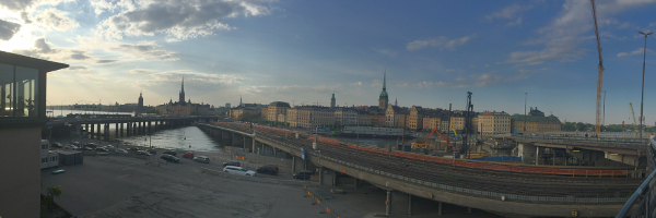
After the classes, Alan and Tran enjoyed walking around Stockholm and seeing the sights, including the Vasa Museum and the Nobel Museum.

Aquaveo provides custom, on-site training for SMS, GMS, WMS, ArcHydro Groundwater, and any other water resource modeling need you have. Organizations can set up shared trainings such as this one, or arrange for the same training for their own employees. You can learn more about our training offerings by visiting our site.

Blog tags: 

Using an SRH-2D Restart File

Do you have an SRH-2D project that is going to take a long time to run? If you don't want your computer tied up for hours, or even days, an SRH-2D project can broken up into smaller model runs that build on each other. This is done by using a restart file or hot start file.

In SRH-2D, a restart file can be specified for the initial wet/dry condition of the simulation. The restart file must have been generated from a previous simulation run that used the same mesh. Several output options exist for creating restart files including: creating them at a regular interval, at a specified list of times, or a single restart file at the end of the simulation.

When SRH-2D does a model run, it creates a series of files for each time step. These restart files are named [casename]_RSTn.dat where n corresponds to the time index. The time series output index file is named [casename]_TSO.dat and holds a list that matches the restart files to a specific time step.

When a restart file is used as an initial conditions hot start file, the previously computed hydraulic conditions from the restart file will always be applied to the start time of a simulation.

To use a hot start condition, do the following:

  1. Run an SRH-2D simulation to completion.
  2. In the output files for the model run, locate the file ending with "TSO.dat" and open it in a text editor.
  3. In the TSO file, locate the time step where you want to use to start your next next simulation run.
  4. In you SMS project, duplicate your simulation.
  5. Open the SHR-2D Model Control dialog for your new simulation.
  6. In the Initial Conditions section, select the Restart File option.
  7. Press the Select button to browse to your restart file.

SRH-2D will now use the conditions from the restart file when you perform your next model run. Now that you know how to use a restart file for an initial condition in SRH-2D, try it in the Community Edition of SMS today!

Blog tags: 

Pages