5 New Features in SMS 13.0 Beta
By aquaveo on October 17, 2018We’re happy to announce the beta version of SMS 13.0 is now available. Our developers have been working hard to improve SMS to make the user experience more enjoyable.
To help you learn about some of the new features, we’ve compiled this list of three new features in SMS 13.0 Beta.
- Notes can now be added to Properties dialog. Right-clicking on most items in the Project Explorer now have a Properties command that will bring up a dialog with a Notes tab. We have found many uses for this, including making notes about the differences between different map coverages or scatter sets.
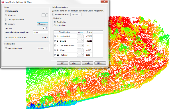
- New tools to support the use of lidar data. You might have used lidar files in the past and noticed that the interface was a little confusing and sometimes slow. After examining how the process could be improved, we made improvements to the import process and changed how SMS interacts with lidar data. We hope you find our new lidar functionality is both faster and makes working with lidar data easier.
- A bridge scour coverage has been added. This allows exporting bridge scour values to the Hydraulic Toolbox to use in analyzing a bridge site. This tool requires having a 2D mesh with elevation data, a water surface elevation, a water depth, and velocity datasets. Most of the values needed will be automatically generated, making bridge scouring faster and easier.
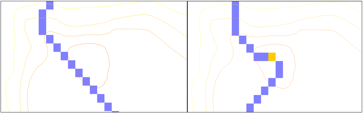
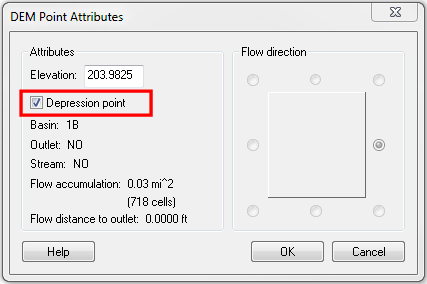
- Floodplain delineation has been improved using the Map Flood tool. This tool allows accessing FEMA data to automatically designate flood areas in your project. The tool can also work with local data provided as a scatter set.
- A 2D scatter set can now be converted into a raster file. Right-clicking on scatter set item in the Project Explorer now has a new Raster -> Scatter command. Creating a raster from your scatter data can help facilitate sharing data across different applications.
These are only some of the many new and updated features in SMS 13.0 Beta. You can find a bigger list of them here. Along with these new features, we are also excited to offer new tutorials instructing users on how to best utilize the new features. Try out the beta by downloading it today!