Generating a 3D Grid from Raster Data
By aquaveo on February 13, 2024Have you heard about the 3D UGrid from Rasters tool that’s new to the Groundwater Modeling System (GMS)? Previous versions of GMS required you to build a raster catalog and then use the “Horizons to Solids” command in order to generate a 3D unstructured grid (UGrid) when modeling stratigraphy. The 3D UGrid from Rasters tool, which is in GMS’s toolbox under the “Unstructured Grids” folder, streamlines this process by allowing the two previously separate processes to be set up in the same place and executed simultaneously.
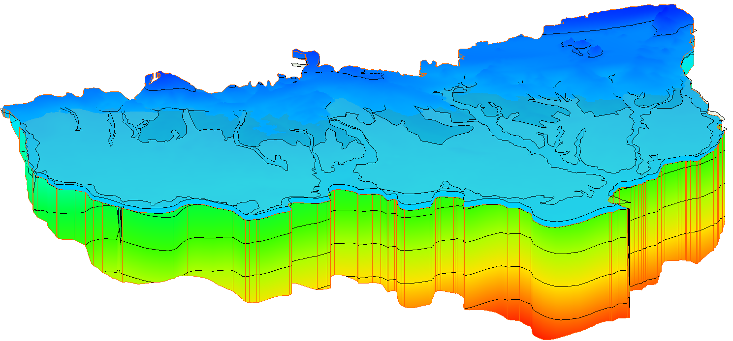
The base components for creating a UGrid with the 3D UGrid from Rasters tool are a 2D UGrid and multiple rasters. The rasters are then added to a table and assigned a horizon number. The term “horizon” refers to the top of each stratigraphic unit that will be represented in a corresponding solid, HUF unit, or 3D mesh layer. Horizons are ordered from the bottom up. For each raster you can choose to fill or clip the layer. Choosing “fill” tells GMS to use the raster to create a UGrid layer. Choosing “clip” tells GMS that any lower surfaces should truncate at that layer. You also have the option of creating sublayers between any rasters that have the “fill” option turned on. You can then set the relative size of each of the sublayers so that they are all proportional, or of differing sizes.
After setting all of the parameters for your UGrid in the rasters table, you then need to set a target location so that GMS knows to calculate elevations at the UGrid cell tops and bottoms or at the points. Lastly, you’ll need to define the minimum thickness that every layer must have, and choose a name for your new UGrid.
If you want more details about how the 3D UGrid from Rasters tool works, you can check out this page of our wiki. You can also look at the newest version of the Horizons with Rasters tutorial.
Head over to GMS, and use this new tool to simplify the stratigraphy modeling process.
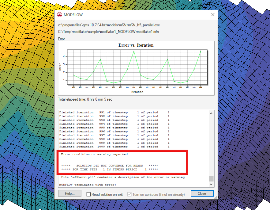 The next thing to look at in your MODFLOW model when you’re trying to figure out what the issue may be is the command line output from the