Aquaveo & Water Resources Engineering News

Isosurface Transparency

For some time GMS has included the ability to have transparent surfaces and transparent contours. These transparent surfaces can come from a TIN, Solid, Cross Section, Mesh, or Grid. The transparency for these surfaces is controlled by adjusting the transparency field in the Material Properties dialog. For contours, the transparency is controlled in the Contour Options dialog.

One of the new features in GMS 9.1 is the addition of transparency for iso-surfaces. The transparency of individual iso-surfaces can be controlled in the Iso-surfaces Options. Below we show the dialog and some iso-surfaces with and without transparency.
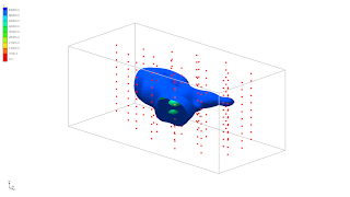
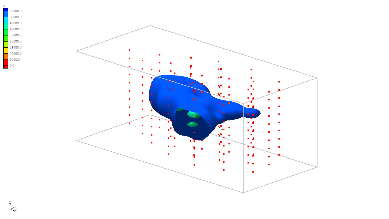
Iso-surfaces without transparency

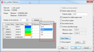
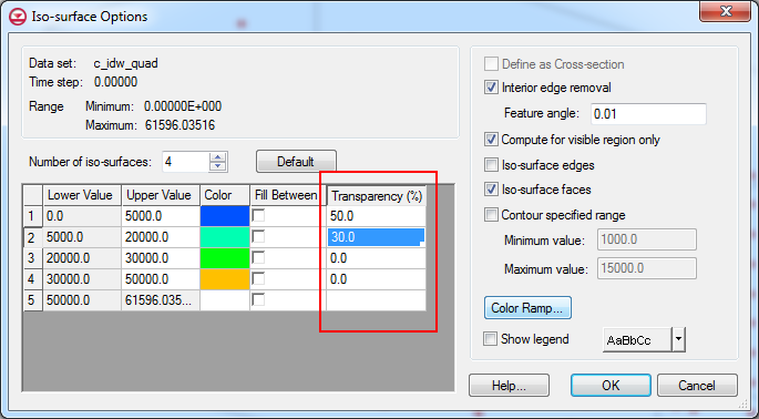
Iso-surface dialog with transparency control

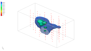
Iso-surfaces with transparency

June 2013 Sprint

  • Fixed 6 bugs
  • Fixed problems with the new "Copy to Coverage" command
  • Updated help links to wiki pages and added automated tests to report when these get out of date
  • Good progress on improving MODFLOW native text output
  • Good progress on open sourcing MODFLOW changes
  • Overhauled MT3D Basic Package dialog to make setting starting concentrations much easier
  • Project-on-the-fly: made new objects get assigned the display projection
  • Sped up test coverage analysis
  • Started work on FEFLOW mesh import/export
  • MODFLOW-LGR progress
  • MODFLOW-USG progress

MODFLOW-LGR

The MODFLOW-LGR interface in GMS is almost done. Here are a couple of images showing a nested child grid in plan view and front view.


MODFLOW-LGR with nested child grid, plan view

MODFLOW-LGR with nested child grid, front view


MODFLOW-USG Progress

The GMS development team has been working on implementing MODFLOW-USG since the documentation was released on May 3, 2013. We have been making good progress. One of the items related to MODFLOW-USG is the ability to work with unstructured grids. The figures below show some of the grids that we have generated with the development version of GMS. We used the same conceptual model and generated a 3D finite element mesh, a 3D structured Grid, and 3D unstructured grids.
Conceptual Model
Finite Element Mesh - FEMWATER or FEFLOW

Finite Element Mesh - FEMWATER or FEFLOW
Structure Grid - Traditional MODFLOW


Structure Grid - Traditional MODFLOW

Unstructured Grid - Nested Grids

Unstructured Grid - Nested Grids
Unstructured Grid - Quadtree


Unstructured Grid - Quadtree

Unstructured Grid - Voronoi

Unstructured Grid - Voronoi
 We will be at the MODFLOW and more 2013 conference this next week. Come by our booth to learn more about new developments in GMS with MODFLOW-USG. We will also have a couple of posters that we are presenting.

GMS Training, Olten, Switzerland

Members of the GMS training team recently completed an onsite training class in Olten, Switzerland from April 22-24. It was an intense 3 day training experience. The small class size allowed the students to be very engaged and learn a lot of material in a short period of time. The day following the training was spent working on the client's groundwater modeling project and applying the principles learned in the training. This type of onsite training is available to clients worldwide at very reasonable price. If you are interested in onsite training, including help with your modeling project, contact training@aquaveo.com.


April 2013 Sprint

  • Fixed 7 bugs
  • Project on-the-fly code improvements
  • Training course in Switzerland 
  • MODFLOW-LGR progress
  • MODFLOW-USG progress
  • Testing coverage analysis progress

March 2013 Sprint

  • Fixed 6 bugs
  • Released GMS 9.1 beta. See the What's New.
  • Added lots of user-request features, including:
    • Snap Boreholes to TINs command
    • Exporting material names/colors/patterns/tranparency
    • Computed flow and Residual flow columns added to the map attribute table for flow observations
    • Iso-surface transparency
    • Copy feature objects to another coverage
    • Activate / Inactivate scatter points command
    • MODFLOW-LGR progress
    • MODFLOW-USG progress
    • New tutorials created:
      • MODFLOW - Transient Calibration Pump Test
      • MODFLOW - Transient Observation Data
      • PHT3D - Ion Exchange And Surface Complexation
      • PHT3D - Transport And Mineral Reactions
    • Project on-the-fly interface improvements
    • Progress on code coverage analysis with tests
    • Much code cleanup and refactoring

    Zoom to Selections, Locate Selections

    Two new commands were added at GMS 9.0: Edit | Locate Selections and Display | Zoom To Selections.

    Locate Selections
    The Locate Selections command is in the Edit menu and results in an animated rectangle which starts from the borders of the graphics window and zooms in to surround whatever is currently selected (grid cells, boreholes etc). This helps you identify where your selections are.

    Zoom To Selections
    The Zoom To Selections command is in the Display menu and causes the graphics window to be framed around the currently selected objects (grid cells etc).

    These commands can make working with large amounts of data a little easier.


    Map->MODFLOW with TINs

    The conceptual modeling approach, first introduced by GMS nearly 20 years ago, is unsurpassed in its flexibility and utility in creating Groundwater Models. Part of the conceptual modeling approach comprises assigning properties to GIS objects that are independent of the numerical modeling grid or mesh. For example, an arc can represent a river; properties can be assigned to the arc so that when the arc is discretized onto the model grid boundary conditions will be created with the appropriate values.


    Upstream and downstream stages can be assigned to the arc; as the arc is discretized onto the grid linear interpolation will occur along the length of the arc so that the river stage will vary from the upstream stage to the downstream stage as shown in the figure below.


    With a transient model, a user can assign time series data to both the upstream and downstream ends of the arc. The user can enter this transient data in the form of a step function as well (constant for a period of time and then the value changes and is constant for another period of time). 


    Then when the arc is discretized to the model grid, the boundary condition property is interpolated spatially (from upstream to downstream) and interpolated temporally (different values for different times in the model).


    At times, instead of assigning values at the upstream and downstream ends of the arc, it is useful to assign a property using a surface. This can be done in GMS using a TIN.


    When the arc is discretized onto the model grid, the boundary condition property will be interpolated from the TIN. These approaches are intuitive and flexible.


    The newest version of GMS will increase this flexibility as TINs with transient data sets can now be associated with arcs (and points/polygons as well). This will give users the option to have a surface that changes with time assigned to a boundary condition property. The times associated with the TIN data set can be in date/time format or relative time format.


    There is a user preference for treating the transient data on the TIN as a step function or as a continuous curve. This option is selected when performing the Map->MODFLOW operation under the Transient TIN data sets section.


    Pages