GMS

Exporting and Importing to MODFLOW 6

By aquaveo on March 6, 2019

In 2018, USGS released MODFLOW 6. This version of MODFLOW uses object-oriented programming to provide support for multiple models within the same simulation. Like many of you, we at Aquaveo were excited to see this new development and started on working on ways for GMS to interface with this new version of MODFLOW.

Did you know that with GMS 10.4 you can export your MODFLOW project for use with MODFLOW 6? This allows you to convert your older or current GMS projects for use with MODFLOW 6. This is just one of the new features in GMS 10.4.

Support has also been added to run MODFLOW 6 from GMS and read the head and flow outputs which may be contoured.

The general workflow process for saving, running, and importing the MODFLOW 6 files is as follows:

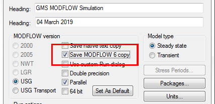
After building your MODFLOW model, open the MODFLOW Global/Basic Package dialog.

In the dialog, turn on the Save MODFLOW 6 copy option under the MODFLOW Version section.
Save your project.
Open MODFLOW | Advanced | Run MODFLOW Dialog... to run the MODFLOW 6 files.
Use the Custom MODFLOW option to point to the mf6.exe executable in program files (e.g., C:\Program Files\GMS 10.4 64-bit\models\mf6\mf6.exe).
Browse to and select the NAM file out of the *_MODFLOW_mf6 folder that will have saved in the same directory as your GMS project. This is not the default, so you will need to browse for it at least the first time.
Run MODFLOW.
Use MODFLOW | Read Solution to select the MFN file out of the *_MODFLOW_mf6 folder.

The exported files can also be used directly in MODFLOW 6.

In the future, we plan to add more MODFLOW 6 functionality to GMS including a full interface. For now, get ready by converting your projects to MODFLOW 6 using GMS 10.4.

Blog tags:

GMS

Creating a Confined Aquifer

By aquaveo on February 6, 2019

Does your MODFLOW model contain a confined aquifer? A confined aquifer layer is defined as "an aquifer below the land surface that is saturated with water. Layers of impermeable material are both above and below the aquifer, causing it to be under pressure so that when the aquifer is penetrated by a well, the water will rise above the top of the aquifer."

In MODFLOW, a layer is considered confined when the head in the cell is above the top of the cell. Additionally, any cell located above the water table will be unconfined because the head in those cells will be below the top of the cell.

The layers in your GMS MODFLOW model can be assigned as confined or convertible in any of the flow packages, such as in the LPF package. Other flow packages can be used as well, including the BCF, HUF, and UPW packages. When setting up the MODFLOW model, select the desired flow package in the MODFLOW Packages dialog. The selected flow package must be compatible with the specified MODFLOW version.

In any of the flow package dialogs, under the Layer Type subheading, a layer can be defined as "Confined" or "Convertible". "Convertible" means GMS will automatically assign the layer as confined or unconfined depending on the elevation of the water table in the simulation. Only one layer type can be assigned to each layer. By default, all layers are set to convertible unless specified otherwise.

When a layer is explicitly set to be confined, MODFLOW will use the thickness of the cell, rather than the saturated thickness, to compute a transmissivity value. It will not check for the unconfined condition in the layer.

After defining the layers as confined or convertible, you will have a confined aquifer for your simulation. Try using confined aquifer layers in your GMS models today!

Blog tags:

GMS

Assigning Elevations in GMS

By aquaveo on January 16, 2019

GMS offers several options for importing, exporting and manipulating elevation data. With so many options, sometimes it can be confusing when choosing which method to use. If you sometimes struggle with elevation data, you’re in luck, because in this blog post we will be exploring different ways that you can utilize your elevation data to accomplish your goals. Listed below are several ways in which you might be interested in using your elevation data.

Assigning elevations in the conceptual model (e.g. to drain nodes)
Using the Select Points/Nodes Tool , double-click on a point/node such as a drain node. This brings up the Attribute Table dialog. Make sure the Feature Type is set to point/node. Here you can set the type of point/node (such as to a drain or a river) and set the bottom elevation. Things such as river arcs and drain nodes require elevations to run the model in MODFLOW.
Interpolating scatter sets/rasters to MODFLOW elevations
Right-click on the scatter set or raster and select Interpolate To and select MODFLOW layers. This will bring up the Interpolate to MODFLOW Layers dialog. Select the dataset you want to interpolate on the left side of the dialog and the layer you would like to interpolate to on the right-side. With both the dataset and the desired layer selected, click Map. This will add the selection to the Dataset=>MODFLOW data queue. Select Interpolation Options if you want to change the interpolation method. Click OK to exit the dialog and interpolate the scatter set to the layer.
Making sure nothing in your conceptual model assigns a polygon elevation that would overwrite the interpolated values
It is important to note that if you have top and/or bottom elevations assigned as areal properties to a polygon, and you map this coverage to MODFLOW, any scatter points or raster elevations previously interpolated to MODFLOW as the top/bottom elevations that lie within the polygon will be overwritten.
Pulling datasets out of MODFLOW (e.g. Layer → 2D Dataset) for manipulation and/or use elsewhere
Another great feature available in GMS is the ability to pull elevations from a MODFLOW layer to create a 2D dataset. This 2D dataset can then be manipulated and/or used elsewhere for various purposes. This can be done in one of two ways; by using the Layer → 2D Dataset option, or by using the MODFLOW Layers to Scatter option.
Layer → 2D Dataset vs. MODFLOW Layers to Scatter (preferred)
It is possible to create 2D datasets from layer arrays in MODFLOW by going to the Global Options in MODFLOW, and selecting the array you want to create a dataset of (starting heads, top elevations, bottom elevations). In the array dialog box select Layer → 2D Dataset or Grid → 3D Dataset. The dataset that this creates will have ids, i, j, and f values.

The preferred method for creating datasets from MODFLOW layers is by selecting the layer and then selecting Grid | MODFLOW Layers to 2D Scatter Points. In the MODFLOW Layers → Scatter Points dialog, you can select to create scatter points within a selected coverage and chose the desired coverage. If you use this option, there must be a polygon in the coverage for the points to map to. This dialog also gives many other options that are extremely useful and convenient. When using this method, the 2D scatter set will have x and y coordinates and the f value.

As you can see there are several ways for you to take advantage of the many options available in GMS when working with elevation data. Whether building from a conceptual model, or maybe even building a conceptual model from a MODFLOW simulation, there are many ways to use your elevation data in GMS. Practice using your elevation data in GMS 10.4 today!

Blog tags:

GMS

Incorporating Geology into a MODFLOW Model

By aquaveo on December 26, 2018

Have you created a MODFLOW model and would like to incorporate geological features in between the MODFLOW layers?

The first step is to create the solid to be used. In GMS, solids are representations of stratigraphy used for site characterization and visualization. Solids can be created in any one of three ways:

Convert horizons to a solid.
Convert one or more TINs to a solid.
Manually create a solid by right-clicking in the Project Explorer and selecting the desired type of solid from the New | Solid menu.

Using the first two methods will allow the solid material composition (what the solid is made of) to be automatically interpolated from the horizon or TIN information. Using the third method will allow you to select the material for each solid reated. The third method also requires knowledge of the XYZ coordinates and other attributes, depending on the type of solid being created (cube, cylinder, sphere, or prism).

Once you’ve created your solids, these steps will integrate the solids into the MODFLOW model:

Right-click on the grid and select Classify Material Zones… to bring up the Classify Material Zones dialog.
Select the solids folder you just created.
Select the Classify algorithm you want to use.
Enter the name of the material set being created.

The Centroid algorithm assigns the solid to the cell if it passes over the centroid of the cell. The predominant material algorithm assigns the solid to the cell if it is the predominant material in the cell (the material making up the highest percentage of the cell). This method maintains your grid, while interpolating the materials to the grid, so that you can have multiple materials within a layer.