Tips for Stochastic Modeling in GMS

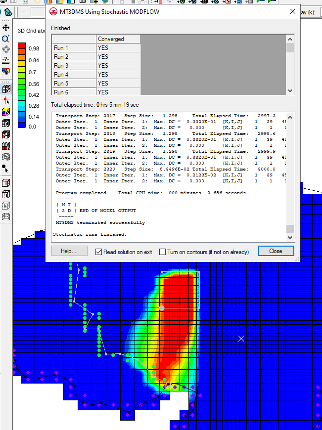
Groundwater models often need to deal with a fair amount of uncertainty, especially when models have limited calibration data available to them. A stochastic modeling approach can be a useful option for dealing with this uncertainty by running a set of models to estimate the probability of certain outcomes, and GMS provides a few tools and methods to utilize this approach. This post will review some tips and tricks when it comes to stochastic modeling in GMS.

GMS provides three methods for stochastic modeling, using either MODFLOW 2000 or 2005. These are parameter zonation (which can be done either by a random sampling approach or a latin hypercube one), indicator simulations, and the Null Space Monte Carlo (NSMC) method.

When parameterizing a model and identifying which model inputs need to be randomized, aim for parameters with the highest uncertainty. But make sure to not select too many parameters, as having too many selected will require substantially large numbers of model runs to complete to be able to sufficiently explore parameter combinations, and this may become unreasonable. Also make sure that when defining key values to parameter zones, you don’t use values expected to normally occur in MODFLOW input. Negative values typically can accomplish this.

When it comes to indicator simulations, T-PROGS software is generally used to generate either multiple material sets or multiple MODFLOW HUF input sets to be used for stochastic simulation. Keep in mind that only a maximum of five materials can be used with the T-PROGS algorithm. This is an intentionally imposed limitation to keep data processing and user-interface from becoming too complex. While it is a hard limit, it is generally easy to condense borehole data down to five materials or less.

Once the stochastic modeling results have been generated, you can refine the results, either with the Risk Analysis Wizard or by using the Statistical Analysis command on a stochastic folder. The latter will create datasets for the mean, min, max, and standard deviation, which can be visualized by using 3D grid display options.

More information on stochastic modeling in GMS can be found at the Aquaveo XMS Wiki or reviewing the GMS tutorials for stochastic modeling.

Try out using stochastic modeling in GMS today!