We use cookies to make your experience better. To comply with the new e-Privacy directive, we need to ask for your consent to set the cookies. Learn more.

Modeling Spatially Varying Flow Resistance
Are you hoping to build more realistic hydraulic models in the Surface-water Modeling System (SMS)? Accurately representing flow resistance across diverse landscapes and materials can be crucial for realistic simulations. This guide will show you how SMS can help you define and apply spatially varying Manning’s n values, capturing detailed differences in terrain like channels, floodplains, and vegetated areas, to enhance your model’s accuracy.
What is Manning’s n?
Manning’s n is a key coefficient in hydraulic models, quantifying the resistance water encounters as it flows over different surfaces. Typical values range from 0.010 (for smooth concrete, pipes, etc.) to 0.150 (for dense vegetation, urban areas, etc.). Applying realistic, varied “n” values significantly improves model accuracy, particularly in complex floodplain and urban drainage simulations.
Defining Materials in SMS
SMS uses material coverages and area property coverages to assign spatially varying Manning’s n values. These coverages consist of polygons over defined project areas that are then further defined with different material types, each with an associated roughness coefficient. This approach allows for detailed representation of surface conditions.
How to Assign Materials
Use the following steps to assign spatially varying Manning’s n values in SMS:
Create a Material Coverage
In the Map Module, right-click on the “Map Data” folder in the Project Explorer and choose New Coverage. Set the coverage type to Material that is compatible with the numerical model you’re using for your project.
Define Material Zones
Create feature polygons to represent different land cover types. The polygons can be created using the create feature objects tools, or through importing GIS data such as shapefiles from land cover datasets (e.g., NLCD). The polygons do not need to be within the grid or mesh being used. SMS will assign the roughness value to the points or elements of the grid or mesh when applied.
A common trick to make defining the materials coverage faster is to duplicate the domain coverage that was used to generate the mesh or grid if you have one. Often the domain coverage has polygons that coincide with the material areas. The duplicated coverage can then be switched to be a materials coverage for assigning materials.
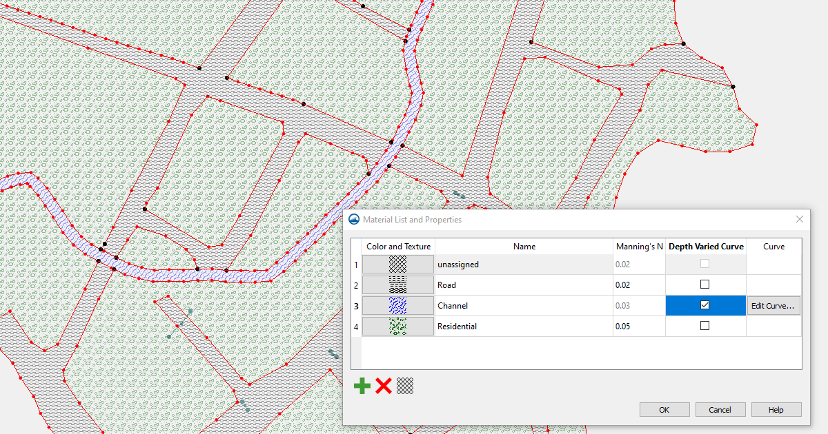
Define Manning’s n Values
Right-clicking on the materials coverage in the Project Explorer will reveal a command to open the materials dialog for that materials type. In this dialog you can create the different materials types and assign the roughness values for each material. Online sources can guide you in selecting reasonable roughness values.
Many models also allow assigning a curve value to the roughness. This permits you to simulate changing roughness values that might occur during the simulation run.
Assign Manning’s n Values
Open the attributes for each polygon on the material coverage and assign a Manning’s n value appropriate for the surface type. Polygons can be left as unassigned which will set the roughness value to the default roughness value found in the materials dialog.
Applying to the Simulation
With the materials coverage defined, transfer the materials values to the computational domain. Use the model-specific linking methods such as applying to the simulation, converting to the grid, or dragging and dropping coverages to assign them.
Check the Assignment
Switch to the Mesh Module (or appropriate grid module) and use the Display Options to color-code the domain by material. This visual check helps verify that all regions were assigned correctly.
Working with GIS Data
SMS supports direct import of standard GIS formats such as shapefiles (SHP) and MapInfo (MIF/MID). These can be used to define polygons for material assignment. When using GIS data, attribute fields can be mapped to material types during import.
Material coverages created in SMS can also be exported as shapefiles for use in other software. For example, a coverage used in SRH-2D can be exported to help define material zones in HEC-RAS cross-sections.
Calibration Using PEST
After assigning initial material values, you can calibrate them using observed data. SMS includes the PEST tool for SRH-2D, which automatically adjusts Manning’s n values within user-defined ranges to improve model accuracy. PEST works by minimizing the difference between computed and observed results. Calibration outputs include observation point plots and error summaries to help evaluate performance.
Take Control of Flow Resistance Modeling
By applying spatially varying Manning’s n values, users can more accurately represent flow resistance across the domain. SMS offers the tools needed to assign, visualize, and calibrate these values using both manual and GIS-supported methods.
Download SMS today to start experimenting with flow resistance!
July 22, 2025
|
View: 3483
|
Categories: SMS
|
By: <a class="mp-info" href="https://aquaveo.com/blog/author/admin">Aquaveo Staff</a>
About the Author

Performing a Silent Install of XMS (Passwords & Hardware Locks)
October 10, 2018
Converting a NET File to an INP File
May 9, 2018
Computing Basin Curve Numbers in 9 Easy Steps
May 16, 2023
Performing a Silent Install for ALS
October 27, 2021
Tips for Finding Information on the XMS Wiki
September 25, 2019
Troubleshooting Projection and Coordinate System Issues
June 23, 2026
How to Determine Soil Texture Using NRCS Soil Data
June 16, 2026
Diagnosing Costly Model Stability Issues
June 9, 2026
New Display Enhancements in GMS 10.9
June 2, 2026
SMS 13.5 Beta Out Now!
May 26, 2026