SMS

Refining Quadtree Grids in SMS

By aquaveo on January 24, 2023

Using the Surface-water Modeling System (SMS), you can model quadtree grids for use with numeric models such as CMS-Flow. Quadtrees are part of the UGrid module in SMS making them a type of unstructured grid. When creating quadtrees in SMS, you can choose to have uniform cell sizes, or you may choose to refine the cells in some areas. When refining a quadtree, there are a couple methods and some tips to keep in mind.

The first method for refinding grid cells in a quadtree is to simply select the cells you want to refine using the Select Elements tool, then right-click and use the Refine Cells(s) command. This will equally divide the cells into smaller, more refined, cells. This method is useful for small-scale refinement in localized areas. However, using this method can be tedious if there are multiple areas on the quadtree that need refinement.

Example of the Quadtree Refinement in GMS

The second method for refining quadtrees is preferred in most cases. This method involves setting refinement parameters in the Quadtree Generator coverage. If you are familiar with SMS’s Cartesian grid generator coverage and mesh generator coverage, you will find that it is similar to both of those coverages.

Like the Cartesian grid generator coverage, the quadtree coverage makes use of a grid frame to define the domain of the generated grid. In the grid frame, you decide the size of the cells in the generated quadtree. It is recommended that this cell size be the largest reasonable cell size for the quadtree grid.

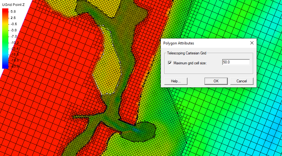
Like the mesh generator coverage, the quadtree generator coverage also makes use of polygons. When you create a polygon on the quadtree generator coverage, you can double-click on the polygon to open the Polygon Attributes dialog. In this dialog you can set the grid cell size for all cells that will be within the polygon.

Using both the grid frame and the polygon attributes, you define how the grid cells are refined for your quadtree with more precision. Try out refining quadtree grid in SMS today!

Blog tags:

SMS

Working with Functional Surfaces for UGrids in SMS

By aquaveo on January 3, 2023

The functional surface option in SMS allows viewing data above a geometry. It has been an option in the 2D Mesh module. The functional surface option has been added for unstructured grids (UGrids) in the UGrid module starting with SMS 13.2. This post will give some guidance and tips for using functional surfaces with UGrids.

Example of a functional surface on a UGrid

Functional surfaces use any dataset as the elevation value for the surface. One of their most common uses is as a representation of the surface of the water above a UGrid. For example, the ocean’s surface in a CGWAVE model. However, functional surfaces can use any scalar dataset to inform the elevations.

A UGrid functional surface gets created by the New Functional Surface UGrid right-click command in the Project Explorer. Once created, right-click on the newly created functional surface to edit the display options. The Functional Surface Options dialog allows you to fine tune the display of your UGrid functional surface. Furthermore, selecting Other Display Options brings up UGrid-style display options.

Once you've set up your functional surface, you may need to make adjustments. Here are some tips on adjusting your functional surface displays depending on your situation:

If your dataset has large numbers, your functional surface might be very tall. To temper that effect, you could set the functional surface Z Magnification between 0 and 1.
If your dataset has very small numbers, your functional surface might appear completely flat. To more clearly see the rise and fall of the data values, set the Z Magnification to a value greater than 1.
If your functional surface is intersecting the UGrid, and you don't want it to, adjust the Elevation Z Offset.
If you want to add contours to your functional surface, click Other Display Options and turn on Face contours. Then click Contours to open the Contour Options.
If you still want to be able to see the UGrid through the functional surface, adjust the transparency. If you're using contours for the functional surface, you'll need to adjust the transparency in the Contour Options dialog.
If you want the functional surface to reference a specific dataset for its elevation, specify a User defined dataset.

Try out functional surfaces with UGrids in SMS today!

Blog tags:

SMS

Computing a Courant Number for an SRH-2D Model

By aquaveo on December 21, 2022

Sometimes, you might want to calculate a Courant number for your SRH-2D model. In most cases, this isn't necessary because SRH-2D is an implicit model. Unlike explicit models such as HEC-RAS, SRH-2D is not Courant limited. With SRH-2D, it is more important to verify convergence and stability than Courant compliance. However, we know that calculating a Courant number dataset for SRH-2D is occasionally desired. Fortunately, SMS now has the Advective Courant Number tool to compute a Courant number dataset based on velocity.

First, let's be clear about what a Courant number does. A Courant number tells you the number of mesh elements that a given water particle passes through during a time step. If the Courant number is less than one, the given particle of water would not pass through an entire mesh element in a single time step.

In SMS, the Advective Courant Number tool computes a Courant Number dataset including every node at every time step. It uses the following equation:

Courant Number Equation

To use the Advective Courant Number tool, do the following:

Make sure a transient SRH-2D solution file is already loaded.
Open the SMS Toolbox, and under Datasets, find the Advective Courant Number tool.
Set the Velocity dataset, the time step length for the simulation, and the desired name for the output dataset.
Run the tool.

Example of the Advective Courant Number tool

The Advective Courant Number tool might stall depending on the vector dataset for your SRH-2D simulation. Running the SRH-2D simulation again might solve this problem. Before running the simulation again, we recommend saving the project as a new file to preserve the old solution files. Then, in the new SMS project file, run SRH-2D again. Once the new solution is loaded into SMS, run the Advective Courant Number tool again using the new velocity dataset.

To see the results, open the Properties dialog for the Courant number dataset. There, you will find the maximum and minimum for the whole dataset and the current time step.

Calculate the Courant number dataset for your SRH-2D simulation in SMS today!

Blog tags:

SMS

Switching Model Executables

By aquaveo on November 30, 2022

The Groundwater Modeling System, Surface-water Modeling System, and Watershed Modeling System (collectively known as XMS) applications make use of multiple numerical models. XMS is packaged with the executables for each of these numerical models. At times, you may need to switch out which numerical model executable XMS uses.

In general, you will want to use the model executable that comes packaged with the XMS. XMS is coded to work with the specific model executables that are distributed with each version of the software.

There are some reasons you might want to change which model executable it used. It might fix a bug with the model executable. It might get you access to features in an older or newer version of the model executable. It might also help you test issues with the numerical model. Replacing the model executable isn't guaranteed to help with any of these, but it is one option for troubleshooting with all of them.

For all XMS applications, the numerical model executables to be used are selected in the Preferences dialog. If you already know where the model executable is, you can copy and paste the executable into the preferences dialog. To do so, use the following workflow:

Copy the executable file path. If using Windows 11, right-click on the desired model executable and select "Copy as Path."
If using Windows 10, open the Properties dialog from the right-click menu. Copy and paste the location path into a text document. Then, make sure to grab the file name ending in ".exe" as well. The executable path will be incomplete without that file name.
In your XMS software, open the Preferences dialog from the Edit menu.
Find the model executable that you want to change and click on the file path next to the name or the Browse button.
In SMS or WMS, this will bring up an Open dialog. In the File name box, paste in the new executable path. If you are using Windows 11, make sure to delete the quotation marks at the beginning and end. Selecting Open saves the new model executable.
In GMS, the model executable is editable without bringing up the Open dialog. Simply erase the former executable path and paste in the new one. As long as the path is a valid path and the path ends in ".exe", GMS will save it. Again, for Windows 11, delete the quotation marks.
Finalize the model executable by clicking OK to exit the Preferences dialog. Otherwise, the executable will not save.

Example of model executables in the Preferences dialog

Now, there are some issues to keep in mind. As mentioned earlier, changing out a numerical model executable is not guaranteed to fix a particular issue or even improve the situation. Older or newer versions of the model executable may not always be compatible with your version of XMS. Sometimes the model executable is not compatible with a particular project. The new executable might even worsen the situation. If any of these things happen, you can reintroduce the original executable.

Check out the available model executables in XMS today!

Blog tags: