Aquaveo & Water Resources Engineering News

Converting an Unprojected Raster to Vector Maps in SMS

In the field of hydraulic engineering, understanding flow dynamics in channels is crucial for effective design and analysis. Converting unprojected rasters with u and v components from a Large Eddy Simulation(LES) model to a vector map in the channel can provide valuable insights. However, this process can be challenging without the right workflow. In this post, we will explore one approach to achieve this in SMS.

  1. Preparing the Data
    To begin, project component rasters to the correct coordinate system. This ensures that the data is in the correct coordinate system for further processing. This can be done in SMS by importing the raster data in the GIS module. Then use the projection command
  2. Importing and Triangulating the Ugrid
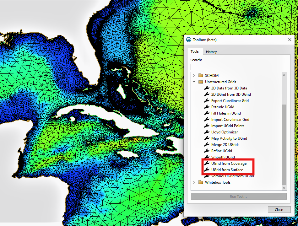
    Next, drag the projected rasters in and convert the u component raster to a Ugrid format using the Raster to Grid tool in the toolbox for SMS 13.2. However, since the resulting Ugrid is created from a raster, the data points are not triangulated for proper interpolation. To address this, select the Ugrid in the project explorer and choose Cells | Triangulate. This allows the data to be interpolated across the surface accurately.
    Alternatively, you can create your own UGrid that encompasses the raster area. Make certain the UGrid has the correct projection.
  3. Incorporating Bankfull Channel Bathymetry
    To add the bankfull channel bathymetry from a raster, interpolate the bankfull elevation to the UGrid points. Use the Data | Map Elevation command to overwrite the existing Z dataset with values from the bankfull dataset. This step ensures that the bathymetry aligns with the UGrid for an accurate representation of the channel.
  4. Example of the Filter Dataset Values tool
  5. Displaying Vectors and Refining the Results
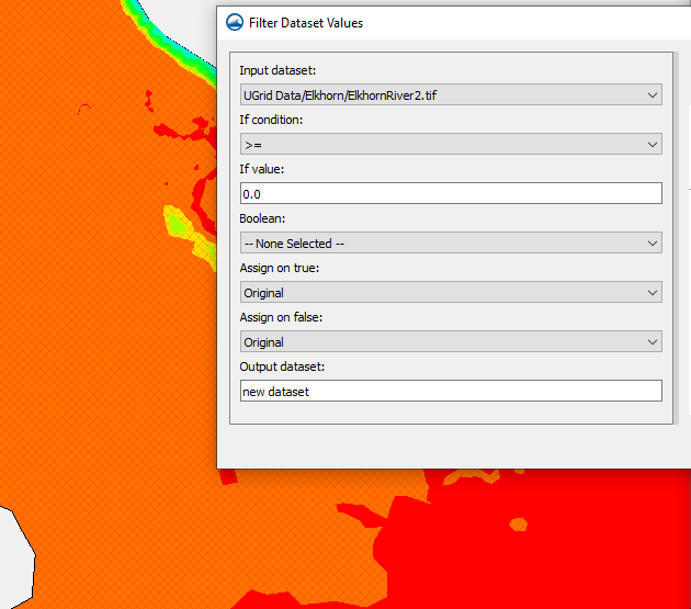
    After combining the u and v components, display the resultant vectors. However, it is common to encounter null vectors outside the channel, which may disrupt the visualization. To address this, utilize the filter and map activities in the dataset toolbox. These tools enable you to mask or remove the null vectors, ensuring a clean representation of the flow hydraulics in the channel.

By following this workflow, you can effectively convert unprojected rasters with components from an LES model to a vector map in the channel using SMS. Proper triangulation, incorporation of bathymetry data, and handling null vectors are critical for accurate visualization of flow dynamics. SMS proves to be a valuable tool in streamlining this process, empowering professionals to gain deeper insights into channel hydraulics and make informed decisions for various engineering applications.

Try out working with raster data in SMS today!

Blog tags: 

New Unstructured Grid Generation Tools in SMS 13.3

The Surface-water Modeling System (SMS) allows use of unstructured grid (UGrid) geometries with multiple numeric models. With that, we have been adding functionality to make generating UGrids easier and more convenient. The toolbox in SMS offers many tools to help speed up UGrid creation and simplify the process. SMS 13.3 beta offers the same tools as before, as well as some new ones. As of now there are fifteen tools under the Unstructured Grids folder in the toolbox. The tool types cover conversion from different types of data to a UGrid, import and export tools, and more. This blog post will explore just two of the many different options in the toolbox.

UGrid creation tools in SMS 13.3

The first UGrid creation tool we will explore in this blog post is the UGrid from Coverage tool. The UGrid from Coverage tool takes the feature objects on a selected coverage and generates a UGrid from the properties of those feature objects. The tool can work with multiple coverage types. Like using the mesh generator coverage to create 2D meshes, the spacing of vertices on the arcs will determine the refinement of the generated UGrid. To generate a UGrid, the coverage must have at least one polygon in it. The parameters required when executing the tool are a coverage, and a name for the new UGrid. We recommend choosing a name that is short, but references the input data for easy reference.

The second UGrid tool we will explore is the UGrid from Surface tool. The UGrid from Surface tool takes an existing mesh, scatter set, or Cartesian grid and creates a new UGrid with copies of all of the datasets. This can be useful because it changes the data into a form that can be modified and manipulated while still preserving the original data. The input parameters include an input mesh, scatter set, or Cartesian grid, and an output grid name. Again, we recommend choosing a name that is short and references the input data.

All of the UGrid tools are accessible by clicking on the toolbox macro at the top of the window, then expanding the Unstructured Grids folder.

Download the SMS 13.3 beta and explore how the UGrid from Coverage and UGrid from surface tools, as well as the numerous other UGrid tools, can help your project today!

Blog tags: 

Understanding the MODFLOW Translator

When importing a MODFLOW file into Groundwater Modeling System (GMS), you may need to translate the file to ensure compatibility with GMS's features and tools. This blog post includes details about the versions of MODFLOW supported by GMS, how GMS uses the translator dialog to transform the MODFLOW file into a version that GMS is able to read and alter, and methods you can use to determine the file version.

Example of the MODFLOW Translator

GMS supports MODFLOW versions 88, 96, 2000, 2005, MODFLOW-NWT, MODFLOW LGR, and MODFLOW USG. However, MODFLOW 88 and 96 are only supported as imports and require conversion to MODFLOW 2000. When importing a MODFLOW file into GMS, if the file was not created in GMS 6.5 or later, translation is necessary for full compatibility with GMS's features and tools, so the MODFLOW Translator dialog will appear. GMS will create a copy of the file before performing the translation which will ensure that the original file is preserved, however you should still always double check that all the data was converted successfully and hasn’t been changed and that none of the data has been lost. During the translation process, you can select the appropriate MODFLOW version from the list provided by the translator for accurate interpretation and conversion.

You can also alter the MODFLOW version inside GMS between supported versions by going to Global Options under the MODFLOW menu. It should be noted, however, that while most versions can be changed back and forth, it can’t be changed back from MODFLOW USG Transport.

There are specific indicators for each version of MODFLOW that can help you to determine what kind of MODFLOW file you are working with if you are unsure which file type it is, which you can view by opening the file as a text file. In a MODFLOW 88 file, the third line of the basic package file contains an IUNIT array with 12 or 24 slots, 24 being the more common option. A MODFLOW 96 file, on the other hand, lacks the IUNIT array and instead features the keyword "FREE" on the third line, indicating that data is in free format, or the third line is entirely blank. Files with a *.dis extension are likely to be MODFLOW 2000, 2005, or NWT models, all of which are supported by GMS.

Certain features and versions of MODFLOW are not supported in GMS. If you have more questions about what MODFLOW features are not supported by GMS, you can follow this link to Aquaveo’s wiki for more information. Head over to GMS and see how this can work for your own MODFLOW models today!

Blog tags: 

Combining Runoff in Watershed Basins with WMS

The Watershed Modelling System (WMS) includes use of the Rational Method, which enables the calculation of peak flows for small watersheds in urban and rural areas. This feature can combine runoff from multiple basins to find the values.

The Rational Method requires a couple specific components to calculate the runoff coefficient for an area. The required inputs are soil data, along with either a table relating soil IDs to runoff coefficients, or a runoff coefficient coverage. Composite runoff coefficients use an area-weighted average of all runoff coefficients that overlay each basin for computation. The inputs chosen will depend on what method you choose to calculate runoff in the Rational Method module. The two primary methods to calculate runoff are first, to assign coefficients to polygons within a coverage, and second, to import a table with all of the coefficients already assigned to a land or soil use ID.

Example of Land Use in WMS Example of Soil Group in WMS

There are two ways to assign runoff coefficients to a polygon. The first way is to enter the coefficients polygon by polygon, and the second is to assign the coefficients through the Soil type mapping dialog.

To assign runoff coefficients polygon by polygon, do the following:

  1. Start with a Runoff Coefficient coverage.
  2. Select one of the polygons that intersects the drainage basin.
  3. Enter the runoff coefficient that matches the soil or land type for that polygon in the Runoff Coefficient dialog window that appears.
  4. After entering the data for each polygon that intersects the basin, activate the Hydrologic Modeling Module and go to Calculators | Compute GIS Attributes.
  5. In the Compute GIS Attributes dialog, make sure the following options are active:
    • “WMS Coverages” is selected as the data type.
    • Under Computation, Runoff coefficients is selected on the dropdown menu.
    • The “Use” dropdown is set to runoff coefficient coverage.
    • The “coverage name” dropdown is set to your new coverage.

To assign runoff coefficients to polygons by soil mapping, do the following:

  1. Start with a “Soil Type” coverage.
  2. Select one of the polygons that intersects the drainage basin.
  3. On the bottom left of the Soil type mapping dialog that appears, turn off the "SCS Soil Type" checkbox and turn on the "Runoff Coefficient" checkbox.
  4. You will now have a list of soil IDs and names with a field for runoff coefficients. Enter a coefficient value for each of these fields according to the material type.
  5. Open the Compute GIS Attributes dialog as described above.
  6. Set everything the same as are in the last set of steps, except change the "Use" dropdown to Coverage.

There are multiple ways to create runoff coefficient tables to import into a project. One of the ways is to create a table from scratch. If you choose this route, you can view the structure requirements on the Aquaveo wiki to make sure it includes everything you need. To import a table with the runoff coefficients, do the following:

  1. With the “Soil Type” coverage active, double-click on a polygon that intersects the drainage basin.
  2. Select “Import file” under Import soil attribute file.

You can also import a table in the Compute GIS Attributes dialog.

Head over to WMS and try out the different ways to assign runoff coefficients to your watershed project today!

Blog tags: