Aquaveo & Water Resources Engineering News

Creating Water Levels in AHGW

When using Arc Hydro Groundwater (AHGW) with ArcMaps, you can create a line that represents a water level, or other structures in your cross section 2D plots. This article will discuss some of the ways to do this.

Inserted water level in ArcMap

If the data is available as a raster surface of water level data, you first call the "Create XS2D Line Feature Class" tool to set up a line feature class for holding the data. Then you will run the Transform Raster to XS2D Line tool, which will insert the line feature for the raster elevation levels that intersect the cross section.

If a raster is not available, you can create a water surface line, but a little more work will be involved.

First, run the Create XS2D Line Feature Class tool once you have the basic cross section set up, to hold the water level line.

Next, you'll have to do one of the following:

  • If you have a general idea of the water level, enter the water level line manually. Manually draw in the water level line, using the Create Features tools built into ArcMap to create polyline features. This is all manually done, and may not match the more detailed data you might have.
  • If you have an image or drawing of the water level for the cross section you're working on, you can insert it behind the XS2D cross section in a way that will match the size and scaling of the cross section. While it is typically used for existing diagrams of cross sections, it could also be used to show the water levels if you happen to have such an image.
  • If you have the water level data as points, you could also add them to an XS2D cross section. This takes point and/or line features with XYZ data and transforms them onto the XS2D cross section. Points at the ground location are used to project onto the XS2D Cross Section, and are given an elevation value based off of a ground elevation raster, not a water level. But, if the water level data is sparse, adjust the values of the water level points to known values (manually), and then follow the first suggestion (manually drawing a line) but snapping the line on these imported points.
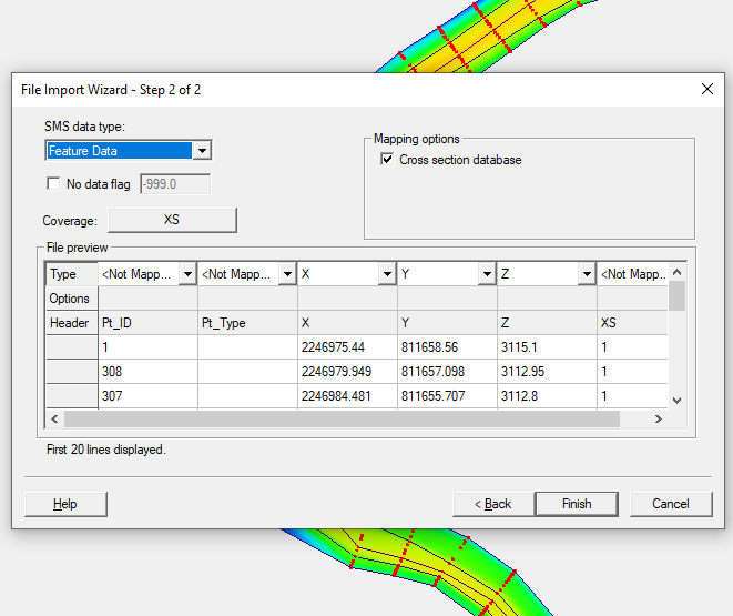
  • Finally, if you have water elevation values at known distances along the line, you could simply import them via a spreadsheet, using the guidelines below:
    • The X value in the XS2D data frame is the distance along the SectionLine feature used to create the XS2D data frame. So if a section line is 1000m long, X=0m is for the start, and X=1000m is for the end. You could automatically calculate this distance if you don't have it by running the Add XY Coordinates (Data Management) tool to get the X values in the attribute table, and then copy them to a spreadsheet.
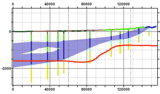
    • The Y values in the XS2D data frame are simply real-world elevation values, multiplied by the Vertical Exaggeration value of the XS2D data frame. For example, if you have a water level of -100m, and a vertical exaggeration of 20, then it will be plotted in the XS2D data frame with a Y value of -2000 (-100 * 20).
    • After getting the X values (distance along the curve), you could simply calculate the Y values as well. If you have depth values, be sure to convert the water levels to elevations, and once you have elevations, multiply by the vertical exaggeration.
    • Then, run the Add XY Data tool in ArcMap. Put the points into an XS2D point layer, and add it to the XS2D cross section data frame. Then make an XS2D line feature class (as mentioned above), and use the create polyline tools to sketch out the water levels (as mentioned above) - basically connecting the dots. When making the line features, make sure that they snap to the points you just created.

Try using AHGW to create water levels or other structures in ArcMap today!

Blog tags: 

Tips for Reprojecting Quadtrees

Are you using a mix of projections or coordinate systems in your SMS project? SMS allows for using data with a variety of projections. That said, when using multiple projections, care must be taken in how the data is imported and incorporated into the project. Issues can appear with mixing certain types of projection units, such as meters and arc degrees. Also, there are limitations for reprojecting certain geometries, such as quadtree grids.

If your project contains a quadtree grid, here are tips for getting the projection of the grid to align with your project projections.

Display Projections for a Quadtree
  1. Make certain that the Display Projection has been set before importing any data or creating any coverages or geometries. Doing this will define the units and projection for any created geometries even though your imported data might be different.
  2. Reproject imported data to match the display projection. A warning will appear about a round-off error, but in most cases the round-off error is not going to affect the final project. It is important to reproject the imported data so that it matches the display projection in order to avoid large errors when running the model. Note that an imported quadtree cannot be directly reprojected, and while it can be used to locate values needed for generating a new quadtree, the imported quadtree should be removed instead of reprojected.
  3. Review all of the data to make certain it aligns correctly. If you have a lot of imported data, this is a particularly important step. You can use the Translate to make minor adjustments if needed, but this is not recommended if there is a large misalignment.
  4. Once you have verified that all of the imported data is aligned, then create the quadtree grid using the quadtree generator coverage. Make certain the grid frame is correctly placed over the imported data. Note that when creating a quadtree, SMS will not extrapolate for areas that are missing data. The newly generated grid will use the same projection as the Display Projection.

After you have a quadtree with the correct projection and unit, you can finish building your project. Having your quadtree in the correct projection significantly reduces the chances of encountering an error with your project.

These tips for using projections and quadtrees can be applied to other projects in SMS. Try them out in SMS today!

Blog tags: 

Tips for Mapping Solids to MODFLOW

Making use of solid models can aid in modeling complex stratigraphy for MODFLOW. GMS allows using solid models to add complexity to your MODLOW projects. The solid module is used to model solids which then need to be mapped to the MODFLOW model for the solids to be included in the MODFLOW model run.

Solids to MODFLOW

When adding solids to your MODFLOW project, the additional complexity can cause issues in the model run. To avoid undesirable outcomes, here are some tips for mapping solids to MODLOW:

  1. GMS contains an advanced option called Set Operations. Generally speaking, Set Operations are no longer recommended methods for creating solids in most cases. It is recommended that you use the horizons approach instead.
  2. Using a Raster Catalog can aid generating solids. The Fill/Clip method will help preserve the same distribution of materials while hopefully addressing any gaps or other instabilities preventing a successful Solids to MODFLOW operation.
  3. If the Solids to MODFLOW command is still experiencing issues, the Classify Material Zones command can be used instead to transfer that material data to the grid. The material that gets assigned can be chosen in one of two ways. It will either be the material that covers the center of the cell or the material that covers the majority of the cell, but only one material can be assigned.
  4. Alternatively, the HUF package can also be used to transfer materials as it allows for multiple materials without splitting the grid layers. However, if there are issues mapping Solids to MODFLOW, you may run into similar issues when attempting to map Solids to HUF.

Solids in GMS provide a great way to add complexity to your MODFLOW model. Try out using solids with MODLOW in GMS today!

Blog tags: 

Changes to Aquaveo Registration

Aquaveo has been updating its registration process to make using our products easier and more secure. The change affects newer versions of our products, specifically GMS 10.5, SMS 13.1, and AHGW 3.5. Going forward, it will be added to all of our products, including WMS.

The new registration uses new codes: Local and Flex codes.

  • Local password: will support virtual machines and remote desktop, but is only good for one machine and cannot be moved from one computer to another.
  • Flex password: acts like a network lock where the license is hosted on your computer and can be used over remote desktop or on a virtual machine. When you want to move the license to another computer, you simply check the license back in and check it out on another machine. There is no hardware to deal with.

By default the software is set to use the newer registration process with newer versions of the software. Local and Flex codes are not compatible with older versions of our software.

In many cases you won't notice a difference with the change to licensing. However, if you encounter an error with your registration or want to use the older licensing process, you can switch back to using the old registration.

  1. Open the newly installed software.
  2. Choose to run it in Community Edition, if the "no license found" dialog appears.
  3. Once the software is open, go to Edit | Preferences.
  4. Click on the Licensing tab.
  5. Check on the box for "Use Legacy Licensing".
  6. Click OK and restart the software.
  7. Then register the software as you have before.
Switching to legacy registration

Currently, we plan on supporting hardware locks and the legacy registration version for at least the next two years. If you want to try out the new registration system, contact our licensing team at licensing@aquaveo.com.

Blog tags: 

Using the Import Wizard to Create a Cross Section Database

Do you have a cross section database that needs to be included in your surface water project? A new feature in SMS 13.1.1 beta allows you to import a cross section database using the File Import Wizard.

A cross section database can be imported from a spreadsheet or a specially formatted text file. To import a cross section database from a spreadsheet or text file, use the following steps:

  1. Make certain you have created a 1D hydraulic cross section coverage in your project. This is needed in order to have a place to store the cross section database.
  2. If using a text file, make certain it is formatted correctly. It should include an XS ID or Station ID column in order to define the points found in each cross section.
  3. Open the cross section database file using any of the methods for opening a file. This will bring up the File Import Wizard.
  4. In the first step of the File Import Wizard, set the fixed width or delimited properties as appropriate for the file.
  5. In the second step of the File Import Wizard, set the data type to be "Feature Data" and turn on the "Cross section database" option.
  6. Also in the second step, assign the columns of the text file to make the station ID, and xyz coordinates. There is also an option for a PT type that allows you to annotate features such as thalweg, left bank, right bank, left toe, right toe, abutment, pier, and so on.
  7. When done with the File Import Wizard, clicking Finish will import the database in your SMS project. It can be reviewed by looking at the arc attributes of the cross section arcs.
The File Import Wizard for importing a cross section database

Once you’ve imported the cross section database, the cross section data is stored in the project file. Try out importing a cross section database into your SMS 13.1 projects today?

Blog tags: 

Plotting Conductance for the DRN Package

Are you looking for a way to contour the conductance of drainage areas in your groundwater model? If you have a large regional model containing areas with a dense drainage network (ditches, tile drainage, etc.), you can scale up this to represent a diffused drainage system. When doing this, there are not only single ditches simulated with the drain (DRN) package, but whole areas. Using GMS, you can create a contour of these drainage areas.

Contoured drain area

To create this contour, use the following workflow:

  1. Go to MODFLOW | Optional Packages | DRN to open the Drain (DRN) Package dialog.
  2. Make sure IJK is selected on the bottom in order to have the drains at their XYZ locations.
  3. Click the top left blank grey box to select all or select and drag to select all the data points.
  4. Copy the data and paste in a word processor such as Notepad++ and save the file.
  5. Back in GMS, select Open File and select the new text file. The text wizard should open up and already have delimited the file, but double check to make sure all the values are correct.
  6. Click Next then change the GMS data type to 3D Scatter points.
  7. If your file included elevations, you can make sure those are not mapped into your project by changing the dataset above to "Not Mapped".
  8. Otherwise, make sure your IJK cell values are matched up with their respective XYZ values and your conductance is set as the "Dataset".
  9. You may have to select the projection for this dataset in order for it to line up with your current project.
  10. You can then go to Display Options, select 3D scatter points on the left sidebar, and then turn on Contours if it has not already been turned on. You can check the contour options to see if the setup and coloring is to your liking.

Completing this workflow should cover all the drain points within the MODFLOW project. Try out contouring drainage areas in GMS today!

Blog tags: 

Using Shapefiles for Stream Arcs in WMS

Shapefiles contain valuable data that can be used for modeling in WMS. If you have an existing shapefile that has arcs that define the streams for the area you will be modeling, you can use that shapefile to define the streams in your WMS project. Doing this can save you from manually having to define the stream arcs manually.

Do use a shapefile for stream arcs in WMS, do the following:

  1. Import or download the shapefile into WMS. The file data will appear in the GIS module. Review the arcs to make certain they align with the stream location.
  2. With the shapefile active, use the Mapping | Shapes to Feature Objects command.
  3. In the GIS to Feature Objects Wizard, map the shapefile to the drainage coverage. If you are using another coverage besides the drain coverage make certain to select the correct coverage in the first step of the wizard.
  4. After mapping the arcs to the drainage coverage, use the Select Feature Arc tool to select arcs along each stream.
  5. Right-click and select the Attributes command to open the Attributes dialog for the selected arcs.
  6. Change the attributes of the arcs to be Streams.
Converting the arcs to stream arcs

After creating the stream arcs, it is recommended that you review the streams to make certain the streams going in the right direction. Use the display option to see the stream arc direction and use the Reverse Direction command to change the direction of arcs.

It is also recommended that you carefully review the arcs that were mapped over to the drainage coverage. Delete any unnecessary arcs and clean up the arcs to improve the performance of the model. It is recommended that stream arcs be merged together except in locations where they branch or where a subbasin is meant to start. Merge arcs by changing a node to a vertex.

Shapefiles can help you build your watershed project in WMS quickly Try out creating stream arcs from shapefiles in WMS today!

Blog tags: 

Using the Compute Derivative Tool in SMS

With the release of the SMS 13.1 beta, a new tool has been added to the Dataset Toolbox. The Dataset Toolbox contains many tools for creating new datasets from existing data in your project. The Dataset Toolbox contains the Data Calculator as well as tools for comparing datasets and completing certain functions.

Among all the tools currently available, the Compute Derivative tool has been added to the Temporal tools in the Dataset Toolbox. In a previous blog post we discussed the other temporal tools if you want to review the function of those tools. The Compute Derivative tool allows you to create a new dataset showing the change from one time step to the next, or the derivative from one time step to the next of an existing dataset.

To access and use the Computer Derivative tool, do the following:

  1. Have a transient dataset loaded into the project.
  2. Use the Data | Dataset Toolbox command.
  3. In the Dataset Toolbox dialog, select the Computer Derivative tool under the list of Temporal tools.
  4. Select the desired dataset to use for the computation.
  5. Select either the Change or Derivative option.
  6. If selecting the Derivative option, also specify the time units.
  7. Enter a name for the new dataset.
Compute Derivative Tool in SMS

The new dataset generated from the Computer Derivative tool will output data in between the existing dataset time steps, resulting in one fewer time steps than the original dataset.

The Compute Derivative tool is only available for data that is in the 2D Mesh module or the UGrid module. Make certain that you have your dataset included in one of these two modules. If you have your dataset in a different module, you will need to interpolate it over to a 2D mesh or UGrid (unstructured grid) before using the Computer Derivative tool.

Try out using the Compute Derivative tool in SMS 13.1 today!

Blog tags: 

Troubleshooting Importing Boreholes in GMS

Have you encountered issues when importing borehole data into GMS? The majority of the time, there are no issues when borehole data is imported into GMS, but occasionally something becomes misaligned. This article will attempt to address some of the common issues that occur when importing borehole data.

The most common issue happens when the borehole data file is formatted incorrectly for GMS. Often this can be fixed when importing the borehole through the File Import Wizard. Selecting the correct options in the File Import Wizard can resolve many issues. However, in some cases the borehole data will need to be reformatted using a spreadsheet program or text editor. If this is the case, follow the recommended borehole file format.

Another issue occurs when importing borehole data happens when the coordinate system for the borehole data does not match the coordinate system for the GMS project. When this happens, all of the boreholes will be unaligned with the project data or it may happen that all of the boreholes will be stacked on top of each other. This latter case typically occurs when the borehole coordinates are in latitude and longitude, but the GMS project is using a projected coordinate system, which would use linear units such as feet or meters.

To fix this issue, the correct projection needs to be set for the boreholes. This is done by doing the following:

  1. In the Project Explorer, right-click on the imported boreholes and select the Projection command.
  2. In the Object Projection dialog, set the projection to match the project projection.

With the correct projection set, the boreholes should line up with the project data.

Setting projections for a borehole

Additional adjustments to boreholes can be made using the Borehole Editor. This is accessed by right-clicking on the borehole and selecting the Properties command. This method is best when only a few boreholes are imported incorrectly. If several or all boreholes were imported incorrectly, it is recommended to review the borehole data and fix any issues before importing into GMS.

For further troubleshooting with importing borehole data, contact our technical support team at support@aquaveo.com. Try out using boreholes in GMS today!

Blog tags: 

Using Evaluation Versions of GMS, SMS, and WMS

Are you wanting to try out GMS, SMS, or WMS, but aren’t quite ready to commit to purchasing a license? Or maybe you have a license, but your maintenance has lapsed and you’d like to check out the new features in a beta version before updating your maintenance?

Aquaveo permits using an evaluation license for its products to permit you to try out our software to see if it will meet your needs. Evaluation licenses are temporary license codes that let you use all the functionality of our software for two weeks.

To receive an evaluation license code, do the following:

Use the evaluation code to register
  1. Download the software you want to evaluate from our downloads page.
  2. After downloading and installing the software, use the Request License button in the Registration Wizard to go to the Software Evaluation Request page on our website.
  3. Fill out the request form and an evaluation license code will be sent to you.
  4. Register the software using the evaluation license code sent to you.

After registering the software with the evaluation code you will be able to use all of the software functionality to determine if the software will meet your water modeling needs. Note that evaluation licenses are only for evaluation purposes and are not intended for creating finished models. It should also be noted that certain third party models, such as TUFLOW or Hydro AS-2D, will still require a separate license in order to fully evaluate them.

After the two week trial period, the license will expire and you will no longer be able to use the software until a paid license code is entered. You are only permitted one evaluation license per product per version.

If you encounter problems with registering an evaluation license, contact our support team at support@aquaveo.com. If you started an evaluation license and were unable to use the license during the evaluation period, contact our licensing team at licensing@aquaveo.com.

Blog tags: 

Pages