Aquaveo & Water Resources Engineering News

Exporting Map Data to a Shapefile

Feature objects in SMS resemble the objects in shapefiles in many ways. Shapefiles are a file format used by many GIS applications. Starting in SMS 13.1, feature objects in SMS can be directly exported into shapefiles.

SMS 13.1 allows points, arcs, and polygons to be exported from a specified map coverage to shapefile. This done by doing the following:

  1. Select the desired map coverage in the Project Explorer to make it active. It is recommended that you hide any map coverages you don’t want exported.
  2. Right-click on the coverage and select Export.
  3. In the Export Coverage dialog, select the direction where you want to save the shapefile, enter the shapefile name, and select which type of shapefile to use.
Exporting a coverage to a shapefile

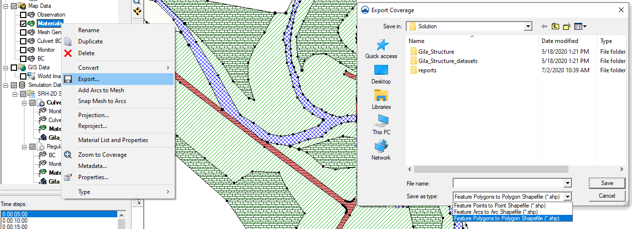
Be certain to select the correct file type when exporting feature objects. Only the matching feature object type will be exported to a shapefile from the coverage. SMS allows you to export feature points as a points shapefile, feature arcs as a line shapefile, and feature polygons as a polygon shapefile.

It is also recommended to review the feature objects on the coverage before exporting to a shapefile. Individual feature objects cannot be exported at this time, therefore, it is advisable to remove any unwanted features before exported. This can be done by duplicating the map coverage and then deleting the unwanted feature objects.

If desired, you can import the exported shapefile into SMS. The shapefile will appear in the GIS module and can then be compared with the feature objects on original map coverage. Otherwise the shapefile is ready to be imported into the desired application.

It should be noted that not all data on map coverages can be exported into a shapefile format. Some data, such as boundary conditions attributes or coverage specific settings, may not end being exported.

Try out creating shapefiles from feature objects in the SMS 13.1 beta today!

Blog tags: 

Tips for Importing Wells to the Conceptual Model

In many MODFLOW projects, having the correct placement and settings for wells is important for getting correct results. GMS facilitates the implementation of wells by allowing well data to be imported directly into the conceptual model. This article gives an overview of importing well data directly into the conceptual model along with some tips.

Importing wells directly into the conceptual model first requires that the wells be in a file with the correct format. Typically this is a text file. Please refer to our wiki article for the correct format that GMS will use.

Other file formats, such as shapefiles, are also common, but often cannot be imported directly into the conceptual model. These other formats will import the wells into a different module, such as the GIS module, and will need to be converted over to the conceptual model.

Before importing well data into the conceptual model, make certain you have an existing map coverage with the well option turned on. Without this, the well data cannot be imported directly to the conceptual model.

When importing well data in a text file, you will use the Open command then the Import File Wizard. In the second step of the File Import Wizard, you must select "Well data" for the GMS data type. Also in the second step, make certain all the data columns are correctly assigned. Failing to assign the data columns correctly can result in errors.

Importing a well file into GMS

It should be noted that you are not limited to the number of data columns you have in the file. Therefore, you can import multiple wells at the same time. You can also import multiple time series or other data applicable to the wells using this method. Please note that while the wells and time series can be defined in the same text file, it is necessary to import the file twice: once to create the wells, and once to assign the time series to the wells. Constant flow rates can be imported at the time of well creation.

Review the well data after it has been imported. That can be done quickly by bringing up the coverage attribute table dialog for the wells. If the data was not imported correctly, minor changes can be made in using the tools in GMS.

Try out importing well data directly into the conceptual model using GMS today!

Blog tags: 

Converting Soil Data to an Index Map

Do you need to add soil data to your GSSHA model in WMS? Soil data is often needed in a rainfall/runoff GSSHA model so that infiltration can be considered in the model. WMS makes this easy by allowing soil data to be converted to an index map.

In order to include soil data in your GSSHA model, there are few steps to follow.

First, you will need a soil data map coverage. Once this coverage has been created you can add soil data directly to the map coverage. Often, you may have soil data located on a shapefile or other source. The soil data on the shapefile needs to be mapped over to the soil data coverage before creating the index map.

Second, the index map will be included with a 2D grid for the GSSHA model in WMS. Make certain you have created your 2D grid and initiated your GSSHA model.

Finally, convert the soil data coverage to be an index map in your GSSHA project. This is done by doing the following:

  1. Use the GSSHA | Maps command.
  2. In the GSSHA Maps dialog, set the soil data coverage to be used.
  3. Click the Coverages to Index Map button.
Soil data converted to an index map

Once you have converted your soil data to an index map, you can use it in your GSSHA model.

When converting soil data to an index map, we do have some tips to make it go smoother.

  • When converting a shapefile to a soil data coverage, make certain that the soil data with the shapefile has been joined to the shapefile.
  • After mapping a shapefile to a soil data coverage, make certain that the soil data mapped over.
  • Check to see if soil covers the entire area of the 2D grid. A warning may appear if the soil data does not cover the area of the 2D grid.

Once your soil data have been successfully converted to an index map, it is ready to be used in your GSSHA model.

Try out using soil data with GSSHA in WMS today!

Blog tags: 

New Map Annotation Tools in SMS 13.1

With the release of SMS 13.1 beta, a new tool has been added to allow you to have additional annotations on feature objects. SMS already provides several options for adjusting how feature objects are displayed, but now more options exist specifically for feature arcs to help make working with feature arcs easier.

Currently in recent versions of SMS, annotations can be added to label arcs. This would let you see the name of specific arcs. The color and thickness of feature arcs can also be changed. Also, specific annotation options exist for specific model coverages, such as the SRH-2D boundary conditions map coverage.

The new map annotations can add a number of new annotations to your feature arcs.With the new annotation tools, the following can also be displayed:

  • An arrow indicating the the direction of the feature arc
  • Tick marks to indicate the distances along the arc
  • The length and number of tick marks can be adjusted along the arc
  • Tick mark labels can be added
  • The font and color of tick mark labels can be changed
Map module annotations in SMS 13.1

These options allow you to quickly see if an arc has been placed in the wrong direction or to check the measurement of an arc. Note that tick marks will use the units set in the project's projection.

To activate the map annotations, do the following:

  1. Open the Map Display Options
  2. Turn on the Annotations option under the Arcs section
  3. Click the Options button next to the Annotations option
  4. Turn on the different the map annotations options in the Arc Annotations Options dialog

Note, with the exception of the tick mark color, that the line width and color are still determined by the other arc display options. The display of the arcs can be adjusted before or after setting the arc annotation options.

Try out the different map annotation options in the SMS 13.1 beta today!

Blog tags: 

Using the SAMG Solver for MODFLOW

Are you needing to use multiple processors to run your MODFLOW or MODFLOW-USG model? Using multiple processors can speed up the model processing time. In order to use multiple processors for MODFLOW in GMS, the SAMG solver provides the means to do this.

The SAMG solver is developed by the Fraunhofer Institute for Algorithms and Scientific Computing (SCAI). It contains a library of subroutines for the highly efficient solution of large linear systems of equations with sparse matrices. SAMG has an advantage in being almost unconditionally numerically scalable. This means that the computational cost using SAMG depends linearly on the number of unknowns.

Before using the SAMG solver, check to see if you have it added to your license. Do this by going to the Register command in the Help menu. Look through the list of components to make certain the SAMG parallel interface / solver has been enabled.

The SAMG solver works with the LMG solver package in MODFLOW. The LMG solver needs to be selected to access the SAMG solver. The LMG solver links the MODFLOW project to the SAMG solver.

SAMG warning message

To activate the SAMG solver do the following:

  1. Open the MODLOW Global/Basic Package dialog.
  2. Then open the MODFLOW Packages dialog.
  3. Turn on the LMG – Link-AMG option.
  4. A warning may appear discussing the SAMG solver. This warning can be turned off if desired.
  5. Once the LMG solver has been turned on, the Link-AMG (LMG) Package dialog can be accessed through the MODFLOW menu in order to set the solver parameters.

Using the SAMG solver is not ideal for all MODFLOW projects. It is generally meant for large linear problems and simulations which use several time steps. For the right project, SAMG can help significantly accelerate the model run time.

For MODFLOW-USG, the SAMG solver is used with the SMS Solver. You can select the SAMG solver in the SMS Solver options.

Contact Aquaveo's licensing team to see about using the SAMG solver with your GMS projects.

Blog tags: 

Editing DEM Elevations

Do you have a Digital Elevation Model (DEM) that has elevations that need to be adjusted? Editing DEM elevations can sometimes prove difficult. However, with WMS you can edit the elevations of DEM files using several tools WMS provides for editing DEM elevations.

Here are a couple ways DEM elevations can be edited in WMS:

Editing Single Points

Some DEMs have a single point where the elevation is off. You can edit a single point in a DEM by using the Select DEM Points tool and selecting the point. You can then edit the point elevation by double-clicking on the point to bring up the DEM Point Attributes dialog where the elevation value can be changed.

Using Feature Arcs to Edit Elevation

Sometimes, the elevation of a DEM needs to be adjusted to follow a specific line, such as a river bed or proposed irrigation channel. The elevation in this location can be adjusted using a feature arc. This is done by selecting the feature arc then right-clicking and selecting the Edit DEM Elevations command.

Editing DEM Elevation using an Arc

In the Edit DEM Elevations dialog, you can change the elevation of the DEM along the arc. This can be done by selecting and changing elevation points on the arc in the profile window. For editing all of the elevation values along the arc, the dialog provides the following options:

  • You can offset all of the arc elevations by using the Offset elevations by a constant button.
  • You can set all of the elevation values to a constant by using the Set to constant elevation button.
  • Finally, you can use the Interpolate button to interpolate the values to between the first and last values on the arc. This will smooth out the elevation to create an artificial slope.

Using these tools makes adjusting the elevations of DEMs easier. Try them out in WMS today!

Blog tags: 

Using the Temporal Tools in the Dataset Toolbox

SMS contains several ways to work with datasets. Perhaps the most useful of these is the Dataset Toolbox. The Dataset Toolbox has several tools for generating new datasets. Among these are the temporal tools which allow adjusting the time steps for a transient dataset. The temporal tools include two options: Sample Time Steps and Merge Dataset.

The Sample Time Steps tool allows the creation of a dataset with a different number of time steps. The time steps can either be increased or decreased. To use the Sample Time Steps tool:

  1. Open the Dataset Toolbox and select the Sample Time Steps tool.
  2. Select the transient dataset you want to use.
  3. Select the starting and end times.
  4. Enter the time step frequency and units.
  5. Give the new dataset a name and click Sample.
Dataset Toolbox showing the Sample Time Steps tool

The other temporal tool is the Merge Dataset tool. This allows us to combine two transient datasets. To use this tool, the transient datasets being combined cannot have overlapping time steps. Most often, this tool is used to append multiple simulation runs together.

For example, if you completed an SRH-2D model run for one day, then created a new simulation for a second day (using a hot start file from the end of the first day simulation run), you could combine the results of the two simulation runs using the Merge Dataset tool.

To use the Merge Dataset tool:

  1. Open the Dataset Toolbox and select the Merge Datasets tool.
  2. Select the first dataset to use, then select the second dataset.
  3. Enter a name for the combined dataset and click Compute.

When using the Merge Dataset tool, make certain that the first dataset selected has time steps that are earlier than the second dataset selected.

The temporal tools in the Dataset Toolbox provide a simple way to adjust transient datasets in your project. Try using these tools in SMS today!

Blog tags: 

The HDF5 File Format and MODFLOW

The HDF5 file format is a cross platform binary format for storing scientific data. HDF5 allows you to reduce the size of the file data by compressing repeated values. This allows your data to be read and written much faster than if you stored the data as ASCII (plain text) files. GMS can read and write to HDF5 files, and stores its own HDF5 files with the other MODFLOW data files.

Exporting an HDF5 file

There are no hard file size limits. The number of objects within an HDF5 file is not limited, and the format supports complex relationships through grouping and linking. In addition to support for common metadata types, you can create user-defined metadata to accommodate whatever needs you have in your project. The only limits with these are the capabilities of your computer.

HDF5 was designed to be extensible and to allow for future changes to the platform. GMS takes advantage of this by checking HDF5 data for key values in order to substitute them into your arrays or lists. This allows you to better use transient parameters and very large pilot point sets. GMS handles the pilot point interpolation through an external routine that helps speed up the processing.

There are external HDF5 file viewers and editors, such as HDFView. However, it is very easy for you to modify the data in such a way that it makes the HDF5 unreadable by GMS. Because of this, we recommend only viewing the files using these tools. You should only manually edit the file if given explicit directions by a developer. If modifications need to be made to the HDF5 file, we recommend you make the changes to your project in GMS which will re-export the HDF5 file.

Learn more about the HDF5 file format from the HDF Group, a consortium of scientists worldwide that works on the HDF5 format. You can also read the article on the XMSWiki about using the HDF5 format with MODFLOW. This article goes into more details about multiple specific uses for the file format.

Make use of HDF5 files with MODFLOW in GMS today!

Blog tags: 

Using Pre-Generated Polygons to Delineate a Basin

Delineating an accurate basin is an important part of a watershed project. WMS provides a number of tools for delineating a watershed basin. The Hydrologic Modeling Wizard is often used to step through the entire process of delineating a basin.

However, it is possible to delineate a basin using data from outside of the Hydrologic Modeling Wizard. In particular, the Drainage module contains tools for delineating a basin using existing project data.

For example, if you have a shapefile with polygons that gives the general outline of the basin, that shapefile can be used to delineate the basin. To use the shapefile polygons to delineate the basin, do the following:

  1. Import the shapefile into WMS. Verify the location is correct.
  2. If you have not already done so, add a DEM for the area of interest to the project.
  3. Generate the flow direction and accumulation, either by running TOPAZ/TauDEM or by importing it.
  4. Map the shapefile polygon(s) into feature polygons in a drainage type coverage.
  5. Place your outlet point(s) and digitize the streams. You can either manually draw the arcs, or load the streams from a shapefile. Be sure to verify that the arcs are set to Stream (not Generic) and that the directions are flowing from upstream to downstream (see "Stream Arrows" in the Drainage Display Options).
  6. Select DEM | Polygon Basin IDs -> DEM in the Drainage module.
  7. Select DEM | Compute Basin Data in the Drainage module.
Basin delineated from shapefile

Once you have a delineated basin, you can use the basin with the watershed modeling model of your choice. Be certain to review the basin to make certain it contains all of the area you need for your project.

WMS provides a large amount of flexibility in delineating a watershed basin in order to adapt to the needs of your project. Try out the different basin delineation tools in WMS today!

Blog tags: 

Viewing Vectors on the Watersurface

With the release of SMS 13.1 beta, a new option has been added to the Vector tab. The existing Vector tab in the Display Options dialog allows viewing vector data as arrows as data points in your project. SMS can change the density of how the vector arrows are displayed and to display the vector arrows along a constant elevation. This new option allows you to display the model vectors relative to a selected dataset.

To use this option:

  1. Open the Display Options, turn on vectors, and go to the Vector tab.
  2. On the Vector tab and change the Origin to be "Relative to dataset".
  3. Select the Dataset button under the Origin to bring a tree item selector dialog.
  4. Select the Dataset you want to use.

After closing out the Display Options dialog, you will be able to see the vectors relative to the selected dataset. For example, if you use a water surface elevation dataset, you would be able to see the vectors relative to the water surface elevation.

Vectors relative to the water surface elevation

This option is available for all modules that allow displaying vectors. This includes the 2D mesh module, Cartesian grid module, quadtree module, and scatter set module.

There is also an option to specify an offset for the selected dataset. For example, you could set the offset to 1 or 2 to get the vectors slightly above the surface. The result would show the vectors mapped 1 or 2 feet above the ground elevation.

Vectors offset from ground elevation

This addition to the vector display option can be used with any dataset in the same module. Therefore, any dataset in the mesh module can be used with a mesh, any dataset in the scatter module can be used with a scatter set, etc.

Try out using the new "Relative to dataset" vector display option in the SMS 13.1 beta today!

Blog tags: 

Pages