GMS

GMS Training in Hannover, Germany

By aquaveo on October 3, 2018

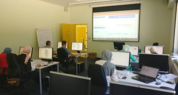
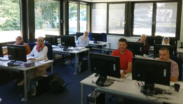
The German Federal Institute for Geosciences and Natural Resources (Bundesanstalt für Geowissenschaften und Rohstoffe, or BGR) hosted a GMS training class in Hannover, Germany from July 31 to August 3, 2018. It was taught by Todd Wood, an Aquaveo consultant, and attended by employees of BGR and the Jordanian Ministry of Water and Irrigation (MWI).

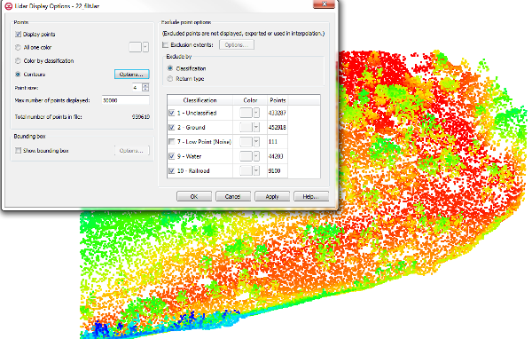
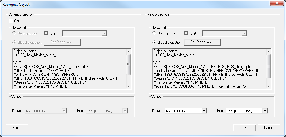
The first day of the four-day training included instruction on the basics of using GMS, including conceptual model development, defining boundary conditions, and the differences between 2D and 3D modeling. Discussion of MODFLOW and its many packages took up the majority of the first day.

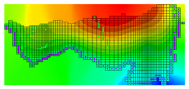
The second day’s training focused on working with regional MODFLOW models (including base maps, conceptual models, and conductance), 2D geostatistics with MODFLOW layer elevations, and interpolation methods. The third day of training covered characterization using borehole data, user-defined cross-sections and horizons, as well as an introduction to model calibration.

The final day of training included automated calibration tools in GMS, including the use of PEST and transient modeling. The day ended with an open lab where participants could work on their own projects with Todd being available to answer questions and help.

We appreciate Falk Lindenmaier and Mark Gropius for arranging the training session for BGR and MWI, and thank you to all of those who attended the training. We love meeting new people and helping them to use GMS more effectively!

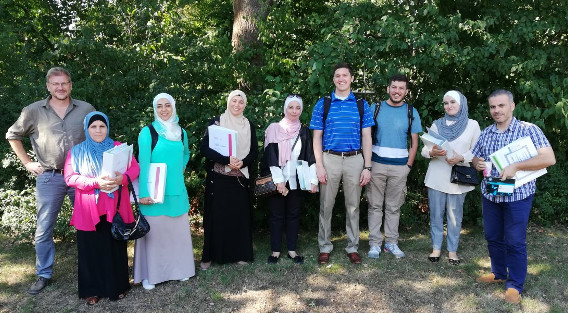
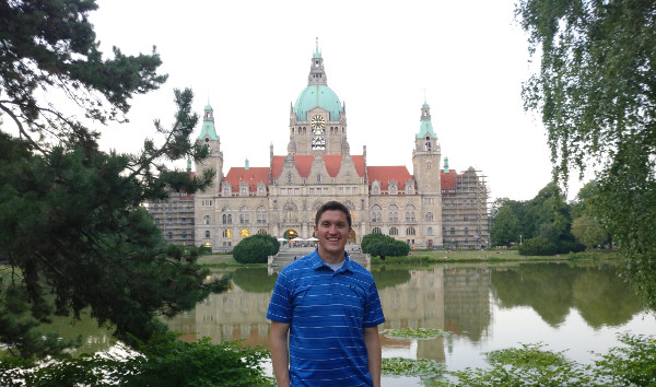
While in Hannover, Todd was able to see some of the sights with those attending the training. They visited the municipal forest known as Eilenriede, the Herrenhausen Gardens, Georgengarten, the Maschsee (an artificial lake), and the New Town Hall. Hannover has some truly beautiful locations.

To arrange your own GMS training session, please see the Aquaveo website.

Blog tags:

GMS

4 New Features in the GMS 10.4 Beta

By aquaveo on September 26, 2018

We’re happy to announce the beta version of GMS 10.4 is now available. Our developers have been working hard to improve GMS to make the user experience more enjoyable.

To help you learn about some of the new features, we’ve compiled this list of four new features in GMS 10.4 Beta.

New tools to support the use of lidar data. You might have used lidar files in the past and noticed that the interface was a little confusing and sometimes slow. After examining how the process could be improved, we made improvements to the import process and changed how GMS interacts with lidar data. We hope you find our new lidar functionality is both faster and makes working with lidar data easier.

MODFLOW-USG Transport can now be used with GMS. This version of MODFLOW allows including transport modeling into your projects. With it comes the Block Centered Transport (BCT) process, Dual Porosity Transport (DPT) package, and Prescribed Concentration Boundary (PCB) package. Other options are also included in the MODFLOW-USG Transport model to give a wide range of access.
Head observations for Connected Linear Network (CLN) wells can now be created to measure the computed head in a CLN node or cell. The process is similar to creating head observations in the groundwater domain with some differences. Overall, CLN observations are simple to create and provide a great addition to the CLN process.
You can now export your MODFLOW project for use with MODFLOW 6. This is done similar to saving native text files.

These are only some of the many new and updated features in GMS 10.4 Beta. You can find a bigger list of them here. Along with these new features, we are also excited to offer new tutorials instructing users on how to best utilize the new features. There are specifically tutorials on the new features listed above. Try out the beta by downloading it today!

Blog tags:

GMS

Creating a Raster from MODFLOW Contours

By aquaveo on September 5, 2018

You’ve just finished successfully running a MODFLOW simulation in GMS and you are viewing the results in lovely contours on your screen. Now you would like to save those results as a raster file you can import into another application.

In order to save the MODFLOW contours as a raster, the MODFLOW results will first need to be converted to a scatter point set, then the scatter point set can be made into a raster.

Converting MODFLOW Layers to Scatter Points

To convert MODFLOW data to scatter point data, do the following:

Select the MODFLOW simulation.
Use the Grid | MODFLOW Layers → Scatter Points menu command.
In the MODFLOW Layers → Scatter Points dialog, you can select the Computed Heads option.
With the Computed Heads option active, you can select the MODFLOW solution datasets and time steps to convert into a scatter point.

Once done, you will have a scatter point set in the Project Explorer containing dataset generated from your MODFLOW results.

Converting Scatter Points to Rasters

Now that you have your MODFLOW solution datasets as scatter point data, you can do the following to convert them into a raster file.

In the Project Explorer under the scatter point set, select the dataset created from the MODFLOW solutions.
Right-click on the scatter point set in the Project Explorer, and select Convert To | New Raster.
In the Scatter → Raster dialog, set the interpolation option you wish to use and specify the extents of the raster.
Finally, save your raster file with a name and raster file type.

The raster file will be loaded into GMS, so you can compare it to the contours in your MODFLOW solution datasets. The raster file contains elevation data that was in the MODLOW solution.

Now that you know how to generate a raster file from MODFLOW contours, try it in out in GMS today!

Blog tags:

GMS

Converting Units

By aquaveo on August 22, 2018

Seeing which units are being used in a project or for a particular object within the project is fairly easy. Converting the units from, for example, U.S. feet to meters, can introduce problems into a project if you do not do it in the correct way.

Reproject

Reprojecting the data involves moving the data from one coordinate system to another. So if your data is in a UTM coordinate system in meters and the rest of your project is in a State Plane projection that uses U.S. survey feet, reprojecting can change the data to match. Conceptually, the data will remain in the same location, but the data will be adjusted to the new units.

To reproject a dataset:

Right-click on the dataset in the Project Explorer and select Reproject.
In the Reproject dialog, the current projection is shown on the left. On the right side, set the new projection and units.

When converting units through reprojection, keep in mind that Z values (elevations) don’t always convert correctly. Round off errors sometimes occur when reprojecting data. In general, reproject does well in changing the X and Y units. The Z value, if it has been set as the bathymetry, typically also converts units well using the reproject option. Other datasets often do not convert between units using the reproject method.

When converting from rasters to scatter sets, the elevation is usually recognized and converted correctly.

Dataset Calculator

Datasets units can be converted using the Dataset Calculator. This is often necessary when the data has been reprojected, but not all of the datasets can be converted using that method. For example, a velocity dataset or conductivity data.

To convert a dataset with the Dataset Calculator:

Select the desired dataset in the Project Explorer.
Select the Data Calculator macro, or the Data Calculator command or the Dataset Toolbox command in the Data menu.
Select the dataset to convert, then multiple or divide the dataset by the conversion value.

There are a few numbers it is useful to have when doing these conversions:

0.304800609601 meters is equal to one U.S. Survey foot
3.28083333333 U.S. Survey feet are equal to one meter
0.3048 meters is equal to one International foot
3.28083989501 International feet are equal to one meter

Note that there are many datasets that will not work with the Data Calculator.

In the end, make certain all the data being used in your model is in the correct units. Having mismatched units will typically create model errors and generate inaccurate results.

Try reprojecting data or using the Data Calculator to convert units in GMS, SMS, or WMS today!

Blog tags:

GMS

SMS

WMS