GMS

Using Exchanges with MODFLOW 6

By aquaveo on March 9, 2022

How can you get models to run smoothly together in MODFLOW 6 in situations where boundary conditions don’t adequately describe their relationship to each other? In MODFLOW 6, you have the option of relating models to each other through an exchange instead of just using boundary conditions. This allows the MODFLOW 6 to calculate the flow between each model as if it were part of one large unstructured grid.

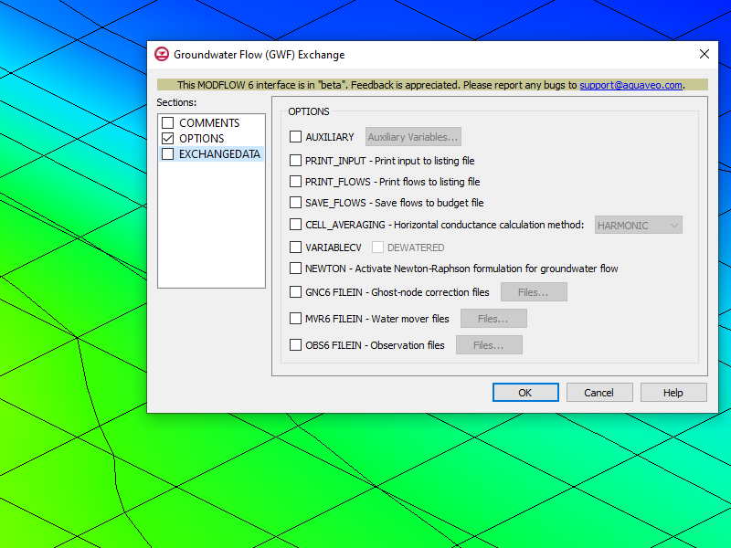
Connecting models through exchanges allows for the transfer of information back and forth between two models with distinct purposes and packages. GWF-GWF Exchanges create relationships between the cells of GWF Models by identifying cells where water will be exchanged between. The GWF-GWT exchange creates a relationship where the GWF Model provides the flow data that informs the GWT Model.

But in what situations might you use these exchanges?

In the case of GWF-GWF Exchange, the USGS has identified several situations where this could be desirable:

Horizontally adjacent models: It may be necessary to connect models that are in the same area in order to better describe how they relate to each other.
Vertically adjacent models: As with the horizontally adjacent models, it may be better to connect models that represent different layers more completely than it is to simply put all the layers on one model. This allows for variation in the fineness of the grids while maintaining communication between them all.
Locally refined grids: You might want to refine grids around areas where you want more specific results. Using an exchange, the simulation will calculate them all like they’re part of the same unstructured grid.
Periodic boundary conditions: This use aims to show the effects of repeating conditions by coupling cells on opposite sides of the model. Instead of exchanging information between cells of adjacent or circumscribing models, you can exchange information between cells in the same model that are not already adjacent to each other.

As mentioned above, the primary purpose of the GWF-GWT exchange is to provide the flow information from the GWF Model to the GWT Model. Since the GWT Model needs flow data for every cell in the model, this is a convenient way to provide that flow data. (For extended information on inputting data for GWT Models, see USGS documentation).

If you have MODFLOW 6 models that you would like to connect to each other, experiment with exchanges in GMS 10.6 today!

Blog tags:

GMS

Having Multiple MODFLOW 6 Simulations in GMS

By aquaveo on February 16, 2022

Have you tried including multiple MODFLOW 6 simulations in your GMS project? Having multiple MODFLOW 6 simulations allows you to run simulations for the same area. This can help with calibration, making comparisons, and troubleshooting a model. This post will cover how to keep things organized when using multiple simulations in a single project file.

After you have created a second MODFLOW 6 simulation, it is recommended that you give the simulation a name that will help you remember the purpose of that simulation. For example if you have a base simulation that you are using to create a stable starting run, it could be named something like “Base_Sim”. If you then create a second simulation that has a longer run time, naming it something like “Base_Longer_Run” might be helpful.

Furthermore, you can use the Notes feature available in the simulation properties dialog to add notes about what makes each of the simulation unique. This can be particularly helpful when sharing the project with coworkers.

In some cases you may have multiple UGrids. For example, you may want to use one UGrid that is less refined for a simulation for a base simulation and a more refined UGrid to test with a duplicate simulation. When doing this, be certain to correctly name the UGrids so that they are easy to tell apart. Also, make certain the UGrid is linked to the correct MODFLOW 6 simulation. It is usually best to create a separate simulation for each UGrid.

Often when using multiple simulations, you will want to have specific map coverages applied to specific simulations. When doing this, you can organize your coverages in the Map module using folders. Using folders can help keep straight which coverages belong with which simulation. And can also help in keeping the Project Explorer from becoming cluttered.

Example of Multiple MODFLOW 6 Simulations in GMS

In the Project Explorer, collapse any folder that you are not currently using. This will help keep the Project Explorer free of any unnecessary clutter. This is particularly helpful when you have solution data from different simulation runs. GMS will automatically place simulation solution files in their own folder in the Project Explorer under the UGrid connected to that simulation, as well as as links under the simulation. Additional folders can be added to organize solution data.

Also, when working with multiple simulations, it can be helpful to lock simulations that are not currently being worked on to reduce chances of accidentally making changes to the wrong simulation.

It should also be noted that having too many simulations in a project can cause GMS to run slowly. It is typically recommended to have fewer than seven simulations in a project.

Having multiple MODFLOW 6 simulations in your project expands your groundwater modeling options. Try out using multiple MODFLOW 6 simulations on your project in GMS today!

Blog tags:

GMS

Defining Hydraulic Conductivity for Specific Layers

By aquaveo on January 26, 2022

In your groundwater model, do you need to define hydraulic conductivity for specific layers differently than other layers? Do you need to modify the hydraulic conductivity values for specific areas within a single layer? GMS provides more than one way to assign hydraulic conductivity. This capability gives you more precision with regard to how hydraulic conductivity is assigned to your groundwater model.

Using the conceptual model approach, hydraulic conductivity can be assigned to polygons on a single coverage then mapped to your model. You can also use multiple coverages, assigning the hydraulic conductivity to specific layers ranges. The workflow for this is as follows:

Right-click on the coverage and select "Coverage Setup...".
In the "Default Layer range" set the layer range you would like to use.

Coverage setup for conductivity on a specific layer

Select the coverage to make it active.
Double-click on a polygon within the coverage.
It will bring up the attribute table for that group of layers.
Set the conductivity for the polygon.
Repeat this process for each desired group of layers.

When using this workflow, take care to make certain you are setting the correct attributes to the correct layer of your grid. Naming the coverage with the layer number or layer range can help with this process. You may also want to use the notes feature to attach reminders as to how the coverage has been set up.

It should be noted that when mapping multiple coverages to your grid, GMS follows an order of priority for the coverages. If you have different conductivity values on different coverages that overlap it is recommended that you apply the coverages individually. The last coverage that you apply will overwrite any overlapping values. If you apply all the coverages at once, the conductivity values will be summed up in areas where they overlap.

Try out using multiple coverages to define hydraulic conductivity for specific layers in GMS today!

Blog tags:

GMS

How to Export Contour Lines as Shapefiles

By aquaveo on January 5, 2022

Have you been wanting to export the contour lines in your GMS project as a shapefile so they can be opened in a different application? GMS allows exporting contour lines as a shapefile. Shapefiles are a file format used by many different GIS software applications. This post will explain how to export contour lines as shapefiles.

GMS contains the Layer Contours → Shapefile command to help save contour lines as a shapefile. Using this command requires your project to be set up correctly. Use the Layer Contours → Shapefile command by doing the following:

Make sure the contours you want to convert to a shapefile are set to Linear in the Display Options. This can be accomplished by opening Display Options and clicking on Contours. In the Contour Method in the top left make certain in the dropdown that it is set to Linear.
Make sure your Grid module is active in GMS, this can be done by clicking on the grid in Project Explorer or selecting the Grid module macro. The grid should be highlighted, meaning that it is now active.
Go to the Grid menu and select the Layer Contours → Shapefile command. Use the dialog that appears to save your shapefile. Be sure to place it in the correct folder and name it properly. Otherwise you might lose the file.
Now open your shapefile in the appropriate GIS software. The contour lines will appear as arc lines.

If you encounter issues with the shapefile, start with checking the folder where you saved the file. Make certain that all of the necessary files for the shapefile are there, including a projection file. Another item to check is that everything you want in the shapefile is displayed correctly in the Graphics Window before you export. Use the display options to adjust the contour lines if needed. Finally, there may be some differences between how GMS displays a shapefile and how other GIS applications display the shapefile. Opening the shapefile in GMS can help you determine if this is the case.

Try out converting contour lines to shapefiles in GMS today!

Blog tags:

GMS