Aquaveo & Water Resources Engineering News

MODFLOW-LGR

The MODFLOW-LGR interface in GMS is almost done. Here are a couple of images showing a nested child grid in plan view and front view.


MODFLOW-LGR with nested child grid, plan view

MODFLOW-LGR with nested child grid, front view


MODFLOW-USG Progress

The GMS development team has been working on implementing MODFLOW-USG since the documentation was released on May 3, 2013. We have been making good progress. One of the items related to MODFLOW-USG is the ability to work with unstructured grids. The figures below show some of the grids that we have generated with the development version of GMS. We used the same conceptual model and generated a 3D finite element mesh, a 3D structured Grid, and 3D unstructured grids.
Conceptual Model
Finite Element Mesh - FEMWATER or FEFLOW

Finite Element Mesh - FEMWATER or FEFLOW
Structure Grid - Traditional MODFLOW


Structure Grid - Traditional MODFLOW

Unstructured Grid - Nested Grids

Unstructured Grid - Nested Grids
Unstructured Grid - Quadtree


Unstructured Grid - Quadtree

Unstructured Grid - Voronoi

Unstructured Grid - Voronoi
 We will be at the MODFLOW and more 2013 conference this next week. Come by our booth to learn more about new developments in GMS with MODFLOW-USG. We will also have a couple of posters that we are presenting.

GMS Training, Olten, Switzerland

Members of the GMS training team recently completed an onsite training class in Olten, Switzerland from April 22-24. It was an intense 3 day training experience. The small class size allowed the students to be very engaged and learn a lot of material in a short period of time. The day following the training was spent working on the client's groundwater modeling project and applying the principles learned in the training. This type of onsite training is available to clients worldwide at very reasonable price. If you are interested in onsite training, including help with your modeling project, contact training@aquaveo.com.


April 2013 Sprint

  • Fixed 7 bugs
  • Project on-the-fly code improvements
  • Training course in Switzerland 
  • MODFLOW-LGR progress
  • MODFLOW-USG progress
  • Testing coverage analysis progress

March 2013 Sprint

  • Fixed 6 bugs
  • Released GMS 9.1 beta. See the What's New.
  • Added lots of user-request features, including:
    • Snap Boreholes to TINs command
    • Exporting material names/colors/patterns/tranparency
    • Computed flow and Residual flow columns added to the map attribute table for flow observations
    • Iso-surface transparency
    • Copy feature objects to another coverage
    • Activate / Inactivate scatter points command
    • MODFLOW-LGR progress
    • MODFLOW-USG progress
    • New tutorials created:
      • MODFLOW - Transient Calibration Pump Test
      • MODFLOW - Transient Observation Data
      • PHT3D - Ion Exchange And Surface Complexation
      • PHT3D - Transport And Mineral Reactions
    • Project on-the-fly interface improvements
    • Progress on code coverage analysis with tests
    • Much code cleanup and refactoring

    Zoom to Selections, Locate Selections

    Two new commands were added at GMS 9.0: Edit | Locate Selections and Display | Zoom To Selections.

    Locate Selections
    The Locate Selections command is in the Edit menu and results in an animated rectangle which starts from the borders of the graphics window and zooms in to surround whatever is currently selected (grid cells, boreholes etc). This helps you identify where your selections are.

    Zoom To Selections
    The Zoom To Selections command is in the Display menu and causes the graphics window to be framed around the currently selected objects (grid cells etc).

    These commands can make working with large amounts of data a little easier.


    Map->MODFLOW with TINs

    The conceptual modeling approach, first introduced by GMS nearly 20 years ago, is unsurpassed in its flexibility and utility in creating Groundwater Models. Part of the conceptual modeling approach comprises assigning properties to GIS objects that are independent of the numerical modeling grid or mesh. For example, an arc can represent a river; properties can be assigned to the arc so that when the arc is discretized onto the model grid boundary conditions will be created with the appropriate values.


    Upstream and downstream stages can be assigned to the arc; as the arc is discretized onto the grid linear interpolation will occur along the length of the arc so that the river stage will vary from the upstream stage to the downstream stage as shown in the figure below.


    With a transient model, a user can assign time series data to both the upstream and downstream ends of the arc. The user can enter this transient data in the form of a step function as well (constant for a period of time and then the value changes and is constant for another period of time). 


    Then when the arc is discretized to the model grid, the boundary condition property is interpolated spatially (from upstream to downstream) and interpolated temporally (different values for different times in the model).


    At times, instead of assigning values at the upstream and downstream ends of the arc, it is useful to assign a property using a surface. This can be done in GMS using a TIN.


    When the arc is discretized onto the model grid, the boundary condition property will be interpolated from the TIN. These approaches are intuitive and flexible.


    The newest version of GMS will increase this flexibility as TINs with transient data sets can now be associated with arcs (and points/polygons as well). This will give users the option to have a surface that changes with time assigned to a boundary condition property. The times associated with the TIN data set can be in date/time format or relative time format.


    There is a user preference for treating the transient data on the TIN as a step function or as a continuous curve. This option is selected when performing the Map->MODFLOW operation under the Transient TIN data sets section.


    Advanced GMS Training, Cairo, Egypt

    Dar Al-Handasah hosted an Advanced GMS Training Course from February 6-12, 2013.


    The class comprised 6 full days of training. A broad range of subjects were covered including: creating MODFLOW models by directly editing 3D Grid, MODFLOW conceptual models, GIS data integration with groundwater models, subsurface modeling, model calibration, PEST, Parallel PEST, SVD-Assist, MODPATH, Transport Modeling with MT3DMS, Stochastic simulations using parameter distributions, Stochastic simulations using TPROGS material sets, Stochastic simulations using PEST Null Space Monte Carlo, SEAWAT, and MODFLOW-CFP. Most of the time in the training was passed using GMS to solve case study problems. Many of the case studies were based on Woburn, MA (the subject of the book and film

    The students really appreciated all of the time spent practicing using GMS to solve a variety of groundwater problems. They especially appreciated how powerful, intuitive, and easy GMS was to work with. By the end of the first day the students were able to create MODFLOW models with almost no help from the instructor.


    Aquaveo wishes to express many thanks to Dr. Abdel-Rahman Abdel-Raouf of Dar Al-Handasah for helping to organize the class.

    On-the-fly projection

    On-the-fly projection is one of the many new features in GMS 9.0. On-the-fly projection means that individual objects (coverages, grids, images etc) can define their own projection. If they do, they will be reprojected to a common display projection when drawn. Thus, if you have data defined in different coordinate systems (state plane, UTM etc) you can now import that data as is and it will all be drawn in the right place. The only necessity is that a .prj file accompanies the data or that you specify the projection in GMS after importing.

    Objects don't have to define their own projection. If they don't, GMS assumes the object's projection is the same as the display projection and just draws it using the object coordinates without performing any reprojection.

    There are a few rules with on-the-fly projection. If an object's projection doesn't match the display projection it cannot be edited. You can, however, change the display projection to match the object's projection, edit the object, and then change the display projection back if you like.

    Another rule is that if a grid (2D or 3D) defines it's own projection, the display projection must match the grid projection. GMS will force them to match. Furthermore, all grid objects (2D, 3D and the grid frame) must either define no projection, or all define the same projection.

    GUI changes

    A number of changes in the GUI were made to support the new projection functionality.
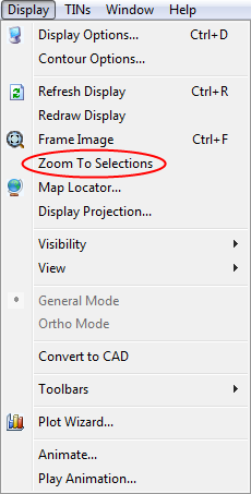
    The Projection command was moved from the Edit menu to the Display menu and renamed Display Projection.

    The status bar was changed to show the current display projection as well as the latitude and longitude whenever the display projection is a global projection:

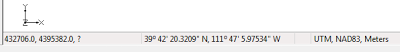
    Status bar showing lat/lon and current display projection.

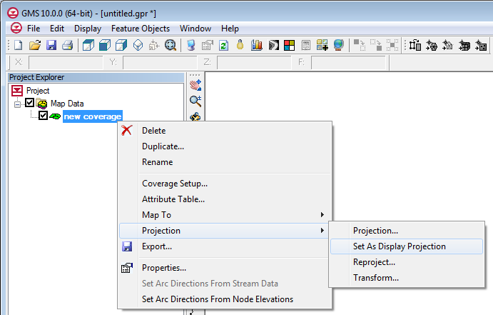
    A standard "Projection" sub-menu was added to the right-click menu of every object. This menu has commands to set the object's projection, set the display projection to match the object's projection, reproject the object, and transform the object.

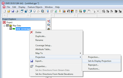
    Standard Projection sub-menu added to all objects.
    The projection dialog was modified so that it now says "No projection" instead of "Local projection". The difference is subtle, but we felt the new verbage was more accurate.

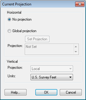
    New Projection dialog.

    Pages