Aquaveo & Water Resources Engineering News

New CityWater Pricing

Are you looking at using CityWater? CityWater is a great way to manage water distribution using cloud-based technology.

Recently, Aquaveo changed its pricing system for purchasing a CityWater license. The old system of standard and professional licensing has been modified. When purchasing CityWater, you can now configure CityWater to meet your needs.

Begin by going to the CityWater Pricing page. This page will show you all of the options that can be included in your license. The top of the page shows the core components included in all CityWater licenses. After the core components, a list of components included with each add-on package is shown. Make a note of the add-ons packages needed for your projects and the number of pipes in your largest project before clicking the Configure button.

On the CityWater License Configuration page, you will select the specific features for your license.

GSSHA

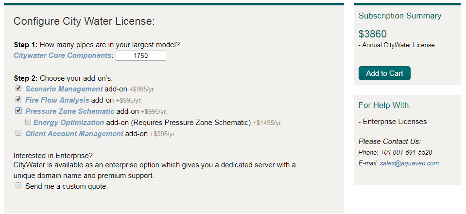
Start with entering the number of pipes in your largest EPANET model that will be used in CityWater. This does not limit the number of models that can be uploaded into CityWater, only the size of model. For example, if your largest EPANET model contains 1500 pipes, you could upload any number of models that contain 1500 pipes or fewer.

If later you find that you need to upload a larger model, contact Aquaveo to receive a quote for adding a larger model.

After entering the number of pipes for your largest model, you can select the packages to add to the license. The components of each package are described in the previous page. If later you discover you need a package that wasn’t originally purchased, contact Aquaveo to receive a quote.

Finally, if you are interested in purchasing an Enterprise License of CityWater, you will need to contact Aquaveo for a customer quote. The price for an Enterprise License depends on the number of additional licenses you will be acquiring and the components of each of those licenses.

When configuring your license, the Subscription Summary will automatically update with a quote based on the number of pipes in your largest model and the selected packages. Clicking Add to Cart will take you to the final page where you can review and pay for your order.

If you have any questions about purchasing CityWater or how CityWater can help you, don’t hesitate to contact us at sales@aquaveo.com.

Blog tags: 

Using the Channel Calculator in WMS

With WMS there is no need to sit and calculate your channel properties by hand, you can use the Channel Calculator to help you obtain the hydraulic data you need. The Channel Calculator, a function of the Hydraulic Toolbox, has the ability to give values for flow, depth, area of flow, wetted perimeter, hydraulic radius, average velocity and so much more. Even better, the Channel Calculator only requires some basic cross-section data including the slope and either the flow or depth of the channel.

This blog post will cover how to compute depths for your channels, which can be used to create floodplain delineation maps, and also how to generate rating curves for your channels, which can be used for things such as predictions. To get started, make sure you have cross-section arcs and river centerlines in your model.

To Compute Depths:

The Channel Calculator is a good tool for approximating channel flows or flow depths. Given a flow rate, the Calculator can compute a flow depth, and vice versa.

  1. In the Hydrologic Modeling Module, select Calculators | Channels to open the Channel Calculations dialog.
  2. Toggle on the Use Cross-Section Database option to enable the ability to import existing cross-section data.
  3. Click the Select Cross Section button to bring up the Assign Cross-Section dialog.
  4. Select your cross-section file along with the cross-section you would like to work with.

The cross section displays in the small graphics window of the Channel Calculations dialog. Adjust the Z scale using the drop-down menu to better visualize the cross section. With the cross section selected, set the necessary parameters to perform calculations for depths.

  1. Click the Launch Channel Calculator button to open the Channel Analysis dialog.
  2. Enter a value for Longitudinal slope. This is an estimate for the ground slope in the vicinity of your cross-section.
  3. Enter a value for the Flow or the Depth depending on which values you have and which ones you are trying to find.
  4. Select the Calculate button. This will populate the right-side of the dialog with hydraulic values calculated for the cross-section.
  5. Select the Create Stage Point button in the Channel Calculations dialog to create a stage point based off the values computed in the channel calculator. This is useful if you are planning to use the depths to delineate a floodplain later on.
To Generate a Rating Curve:

The Channel Calculator can also be used to create different rating curves, to be used to calculate things such as storage potential.

  1. Click on the Launch Channel Calculator button to open the Channel Analysis dialog.
  2. Select the Compute Curves button to open the Curve Selection dialog.

The default is to create a rating curve for the entered flow vs. depth for the selected cross section, but it’s possible to also create curves for all of the other options listed.

  1. When exiting the Curve Selection dialog, the selected rating curves are generated and the plot shouldappear.
  2. If you double-click in the rating curve plot window a dialog will appear that presents many different options for how you can use the rating curve, including an option to export the curve in a chosen format.

As you can see, with just a few steps, you can obtain the hydraulic data you need for your channels in WMS. Try it out today!

Blog tags: 

Saving Plots in SMS

After working to put together the perfect plot for your model to show what is going on, it’s nice to be able to keep that plot. Starting in SMS 13.0, you can save plot parameters with your project or for use in other projects.

Previously, SMS allowed exporting the plot as an image or text file, but it did not allow you to save a plot file that SMS could read to regenerate the plot in your project. Saving a plot allows the plot parameters to be used over and over again, saving you from needing to recreate the plot in the future.

To save a plot, do the following:

  1. After generating a plot, use the File | Save As command.
  2. In the Save As dialog, change Save as Type to “Plot File (*.plt)”.

Furthermore, if a plot window is open in SMS when you save your project, a PLT file will be generated to go with your project.

The PLT file that is generated can be opened in any instance of SMS. The file records the parameters used to generate the plot such as the selected datasets, observation arcs used, and plot display options.

GSSHA

Once the plot file has been saved, opening the file in SMS will regenerate the plot. SMS will attempt to recreate the conditions that existed in SMS when the plot was first saved. If the plot is imported into the same project where it was generated, it should appear the same.

If the plot is imported into a different project, SMS will try to match the conditions as closely as possible. For example, if the plot uses an observation arc, SMS will use the first observation arc it can find. If a mesh was used, then SMS will look for the same mesh. It will also look for the same dataset and if it cannot find it, then it will look for a dataset with the same name.

Test out saving plots in SMS 13.0 today!

Blog tags: 

Creating a Confined Aquifer

Does your MODFLOW model contain a confined aquifer? A confined aquifer layer is defined as "an aquifer below the land surface that is saturated with water. Layers of impermeable material are both above and below the aquifer, causing it to be under pressure so that when the aquifer is penetrated by a well, the water will rise above the top of the aquifer."

GSSHA

In MODFLOW, a layer is considered confined when the head in the cell is above the top of the cell. Additionally, any cell located above the water table will be unconfined because the head in those cells will be below the top of the cell.

The layers in your GMS MODFLOW model can be assigned as confined or convertible in any of the flow packages, such as in the LPF package. Other flow packages can be used as well, including the BCF, HUF, and UPW packages. When setting up the MODFLOW model, select the desired flow package in the MODFLOW Packages dialog. The selected flow package must be compatible with the specified MODFLOW version.

In any of the flow package dialogs, under the Layer Type subheading, a layer can be defined as "Confined" or "Convertible". "Convertible" means GMS will automatically assign the layer as confined or unconfined depending on the elevation of the water table in the simulation. Only one layer type can be assigned to each layer. By default, all layers are set to convertible unless specified otherwise.

When a layer is explicitly set to be confined, MODFLOW will use the thickness of the cell, rather than the saturated thickness, to compute a transmissivity value. It will not check for the unconfined condition in the layer.

After defining the layers as confined or convertible, you will have a confined aquifer for your simulation. Try using confined aquifer layers in your GMS models today!

Blog tags: 

Using GSSHA Group Files in WMS

GSSHA Group files in WMS allow multiple GSSHA projects to be saved together in one set of files. It can sometimes be helpful for you to run GSSHA on multiple related projects in order to compare the results.

GSSHA

You can open multiple projects into one WMS session by doing the following:

  1. Open the first project using the GSSHA | Open Project File option.
  2. Open the second, third, ect., project using the same menu.

Once the desired projects are open in WMS, you can save them as a GSSHA Group Project (GGP) file. This keeps everything together in one location.

  1. Save the project as a group by using the GSSHA | Save Group option.
  2. Select the projects to include in the group.
  3. Give the group a file name.

GSSHA can be run on a group file if you do the following:

  1. Select the GSSHA | Run GSSHA Group option.
  2. Select the projects to run.
  3. Give the project a name.
  4. Select whether to suppress screen printing and/or to import the solutions when the GSSHA run finishes.

When GSSHA finishes running on the first project, the Model Wrapper dialog will automatically close. A few moments later, another instance of the Model Wrapper dialog will appear as GSSHA runs on the second project. This one will also automatically close. This continues this way through all of your selected projects. WMS will then import the solutions from the GSSHA runs.

All of the tips here require you to be in the 2D Grid Module—there are additional GSSHA menus in other modules. Additionally, warnings may appear asking if land use and soil type tables should be overwritten. This is up to your discretion. Keep in mind, however, that it is generally best to import projects in an additive manner, with the most simple project being imported first and the most complex project being imported last.

Try out saving and running GSSHA groups in WMS today!

Blog tags: 

How to Relax or Refine a Mesh in SMS

Are you ever tempted to refine your mesh after creation using the mesh editing tools? Manually changing hundreds or thousands of mesh elements using the mesh tools can be very time consuming.

Although possible to use the mesh tools, it is better to recreate a new mesh when wanting to refine or relax the elements. This will maintain the accuracy of your mesh, and reduces possible issues that may arise later on in the project due to inconsistencies that editing manually creates.

To recreate a refined or relaxed mesh:

  1. Create a mesh generator coverage.
    1. If the existing mesh was created from a mesh generator coverage, you can use that coverage or a duplicate of that coverage.
    2. If a mesh generator coverage does not exist, you can create a mesh generator coverage by converting the mesh boundary or nodestrings to a new mesh generator coverage.
  2. Go to your mesh generator coverage and redistribute the vertices so that there are either more or less arc segments depending on what you are trying to accomplish with your model. To relax the mesh, fewer arc segments are desired, and to refine the mesh more arc segments are desired.
  3. Assign the desired meshing type (paving, patch, etc.) to the polygons in the mesh generator coverage and set the bathymetry source to use. Be certain to preview how the mesh will generate with the new spacing for each polygon.
  4. Now generate a new 2D mesh using the edited mesh generator coverage.
  5. Add the new mesh to your model simulation and run the model using the relaxed or refined mesh.

Sometimes you might not want to relax ro refine the entire mesh. To only relax ro refine part of the mesh do the following.

  1. Create a new mesh generator coverage.
  2. Create a polygon in the area of the mesh you wish to relax or refine.
  3. Redistribute the vertices along the arcs in the polygon to so there is a great or fewer number of segments along each arc.
  4. Set the meshing type for the polygon and assign it a bathymetry source. Be certain to preview the mesh for the polygon to be certain you are getting the mesh you want.
  5. Generate a new 2D mesh for the area being refined or relaxed.
  6. Select both 2D meshes and merge them together.
  7. Add the new merged mesh to your model simulation and run the model.

Using these steps when editing a mesh can make a huge difference in your model and save you time. Try out relaxing and refining meshes in SMS today!

Blog tags: 

Assigning Elevations in GMS

GMS offers several options for importing, exporting and manipulating elevation data. With so many options, sometimes it can be confusing when choosing which method to use. If you sometimes struggle with elevation data, you’re in luck, because in this blog post we will be exploring different ways that you can utilize your elevation data to accomplish your goals. Listed below are several ways in which you might be interested in using your elevation data.

  • Assigning elevations in the conceptual model (e.g. to drain nodes)

    Using the Select Points/Nodes Tool , double-click on a point/node such as a drain node. This brings up the Attribute Table dialog. Make sure the Feature Type is set to point/node. Here you can set the type of point/node (such as to a drain or a river) and set the bottom elevation. Things such as river arcs and drain nodes require elevations to run the model in MODFLOW.

  • Interpolating scatter sets/rasters to MODFLOW elevations

    Right-click on the scatter set or raster and select Interpolate To and select MODFLOW layers. This will bring up the Interpolate to MODFLOW Layers dialog. Select the dataset you want to interpolate on the left side of the dialog and the layer you would like to interpolate to on the right-side. With both the dataset and the desired layer selected, click Map. This will add the selection to the Dataset=>MODFLOW data queue. Select Interpolation Options if you want to change the interpolation method. Click OK to exit the dialog and interpolate the scatter set to the layer.

  • Making sure nothing in your conceptual model assigns a polygon elevation that would overwrite the interpolated values

    It is important to note that if you have top and/or bottom elevations assigned as areal properties to a polygon, and you map this coverage to MODFLOW, any scatter points or raster elevations previously interpolated to MODFLOW as the top/bottom elevations that lie within the polygon will be overwritten.

  • Pulling datasets out of MODFLOW (e.g. Layer → 2D Dataset) for manipulation and/or use elsewhere

    Another great feature available in GMS is the ability to pull elevations from a MODFLOW layer to create a 2D dataset. This 2D dataset can then be manipulated and/or used elsewhere for various purposes. This can be done in one of two ways; by using the Layer → 2D Dataset option, or by using the MODFLOW Layers to Scatter option.

  • Layer → 2D Dataset vs. MODFLOW Layers to Scatter (preferred)

    It is possible to create 2D datasets from layer arrays in MODFLOW by going to the Global Options in MODFLOW, and selecting the array you want to create a dataset of (starting heads, top elevations, bottom elevations). In the array dialog box select Layer → 2D Dataset or Grid → 3D Dataset. The dataset that this creates will have ids, i, j, and f values.

    The preferred method for creating datasets from MODFLOW layers is by selecting the layer and then selecting Grid | MODFLOW Layers to 2D Scatter Points. In the MODFLOW Layers → Scatter Points dialog, you can select to create scatter points within a selected coverage and chose the desired coverage. If you use this option, there must be a polygon in the coverage for the points to map to. This dialog also gives many other options that are extremely useful and convenient. When using this method, the 2D scatter set will have x and y coordinates and the f value.

As you can see there are several ways for you to take advantage of the many options available in GMS when working with elevation data. Whether building from a conceptual model, or maybe even building a conceptual model from a MODFLOW simulation, there are many ways to use your elevation data in GMS. Practice using your elevation data in GMS 10.4 today!

Blog tags: 

Converting CAD Data to Feature Objects in WMS

CAD data has been around for a long time and it’s one of the most readily available formats for geological data. WMS can make use of the data in a variety of ways. One of these ways is to convert CAD data into feature objects.

When CAD data for an area is available, DWG and DXF file data can be automatically converted to feature objects in WMS. Lines, points, and polygons in the CAD file can be turned into feature objects on a Map coverage for use in your WMS projects. This is done by doing the following:

  1. Import the CAD data into WMS. It will appear in the Project Explorer.
  2. In the Project Explorer, right-click on the CAD file and select CAD to | Feature Objects.
  3. In the CAD → Feature Objects dialog, select the layers to be converted to feature objects.
  4. Next, in the Clean Options dialog, select options to clean up the feature objects such as removing dangling arcs.
  5. Finally, the Properties dialog will appear letting you designate the type of coverage that will hold the new feature objects.

After you have converted your CAD data to feature objects, there are few items to keep in mind.

  • Typically, CAD data will not designate the stream direction. Make certain to check the direction of arcs generated from CAD data. Use the Reorder Streams command to fix this.
  • Polygons will not be automatically generated from polygons in the CAD data. Any enclosed arcs must be converted to polygons using the Build Polygons command.
  • It may be necessary to use the Clean Options dialog again after conversion.
  • Additional adjustments to the arcs may be necessary using the Map module tools.

Generating feature arcs from CAD data can save you a lot of time and frustration when building your watershed model. Try out converting CAD data into feature objects using WMS today!

Blog tags: 

Moving SRH-2D Material Attributes to Another Project

After setting your SRH-2D material attributes in one SMS project, have you ever wanted to transfer those attributes to another SMS project? Doing this can save you from having to reenter the same material attributes into a separate project. You can even transfer multiple material coverages at once.

There are three project files referred to here: the original project, the project with the saved material coverage attributes, and the third project to which you want to add the saved material attributes. To make sure these instructions are clear, we'll call them Project A, Project B, and Project C, respectively.

To save time on other projects that use the same material attributes, you can use the following steps to export them for later use:

  1. Outside SMS, create a copy (Project B) of your project directory. This prevents you from accidentally damaging the original project (Project A) during the process.
  2. In Project B (the copy), delete any geometric data that isn’t going to be transferred, such as meshes, grids, GIS data, and scatter sets.
  3. Also remove any coverages and material data you do not want transferred.
  4. On the SRH-2D material coverages, remove any polygons and feature objects that you do not want transferred. This is assuming that the project receiving the new material parameters will be assigning the material properties to different polygons.
  5. This is the tricky part. You have to have at least one Map object for a map file to be saved in SMS. Therefore, create a new coverage of any type as a placeholder. Create a single feature point in this placeholder coverage.
  6. Use the Save command to save Project B that only contains the SRH-2D material coverages with your material properties, and one one other coverage with a single feature object.
  7. In another instance of SMS, open Project C.
  8. Use the Open command to open Project B.
  9. SMS should ask if you want to delete this data. If this happens, respond "No". The coverages from Project B (and its material lists and attributes) will be loaded into Project C.
  10. Now to add the material lists from the Project B into the material lists in Project C by right-clicking on the transferred coverage and selecting the Assign Materials to menu command. SMS will bring up the Assign Materials dialog where you can add materials from one coverage to another. You can either add the materials to the list of this coverage or replace the materials list in this coverage.

Now that you know how to transfer material parameters from one project to another, try it out in the SMS today!

Blog tags: 

Incorporating Geology into a MODFLOW Model

Have you created a MODFLOW model and would like to incorporate geological features in between the MODFLOW layers?

The first step is to create the solid to be used. In GMS, solids are representations of stratigraphy used for site characterization and visualization. Solids can be created in any one of three ways:

  1. Convert horizons to a solid.
  2. Convert one or more TINs to a solid.
  3. Manually create a solid by right-clicking in the Project Explorer and selecting the desired type of solid from the New | Solid menu.

Using the first two methods will allow the solid material composition (what the solid is made of) to be automatically interpolated from the horizon or TIN information. Using the third method will allow you to select the material for each solid reated. The third method also requires knowledge of the XYZ coordinates and other attributes, depending on the type of solid being created (cube, cylinder, sphere, or prism).

Once you’ve created your solids, these steps will integrate the solids into the MODFLOW model:

  1. Right-click on the grid and select Classify Material Zones… to bring up the Classify Material Zones dialog.
  2. Select the solids folder you just created.
  3. Select the Classify algorithm you want to use.
  4. Enter the name of the material set being created.

The Centroid algorithm assigns the solid to the cell if it passes over the centroid of the cell. The predominant material algorithm assigns the solid to the cell if it is the predominant material in the cell (the material making up the highest percentage of the cell). This method maintains your grid, while interpolating the materials to the grid, so that you can have multiple materials within a layer.

Try adding solids to your MODFLOW models in GMS today!

Blog tags: 

Pages