Aquaveo & Water Resources Engineering News

Using SRH-2D Initial Conditions

Are you wondering which initial hydraulic condition to use for your SRH-2D model in the Surface-water Modeling System (SMS)? Setting the initial condition for how each cell is to be treated in an SRH-2D simulation is an integral part of the model. This blog post will explore each of the five options for the initial conditions of a simulation that SMS provides. The settings for the initial conditions are found in the SRH-2D Model Control of the simulation on the General tab.

Example of SRH-2D initial conditions in SMS

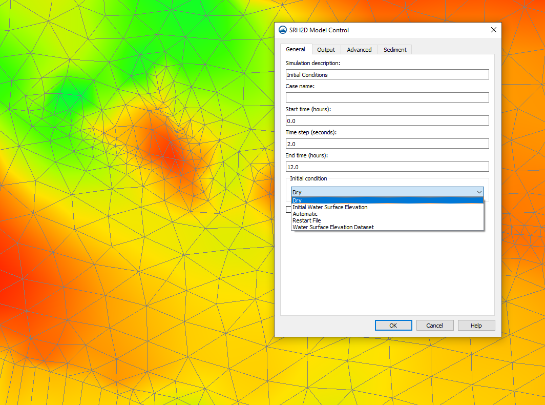
The "Dry" initial condition is the default in SMS. This condition means that there is no water in any of the elements. This selection works well for almost any simulation and is recommended as a good option for the base of an SRH-2D project if you are not certain which condition will suit your project best. The dry condition is also commonly used to create a restart file, which will be covered later.

The "Automatic" condition begins the simulation with water at the outflow depth specified in the boundary condition coverage, which fills the domain. The outflow depth is assumed to be anything lower in elevation than the elements marked as containing backwater. Anything above the backwater elements are marked as dry. Dry and automatic are the best options to use to prepare a restart file condition.

The "Initial Water Surface Elevation" condition takes a water surface elevation dataset and applies one elevation value to all elements. If the starting elevation of an element is higher than the assigned water surface elevation, SMS automatically marks that element as dry. The Initial Water Surface Elevation condition is similar to Automatic in this way, but it can be useful if the water surface elevation value you want to use for your project is different from the elevation at the outflow boundary.

The "Water Surface Elevation Dataset" condition takes the values from a dataset at a single time step to determine the water surface elevation value for each element at the start of the simulation. Unlike the Initial Water Surface Elevation condition, the elevation value at each element will vary. In order to use a water surface elevation dataset condition, a simulation will need to have already been run.

The "Restart File" condition allows you to upload a file from a previous run that contains the initial conditions. This is a quick way to split a particularly long simulation into smaller chunks, which will cut down on run time. Each time SRH-2D runs with any of the initial conditions listed above, a restart file is written and saved to the data files folder outside of SMS. It should be noted that a restart file has to have been generated from a mesh that exactly matches the mesh in the simulation, otherwise it will not work. The slightest difference in the restart file mesh and the simulation mesh will generate an error during the model run.

When a restart file is used to denote the initial conditions, the hydraulic conditions that were computed during the run that created the restart file will always be applied starting at the very first time step in the simulation. More in depth information on the usage of a restart file in SRH-2D can be found in this blog post.

Head on over to SMS and explore the different ways these initial condition options can help you with your SRH-2D project today!

Blog tags: 

Utilizing PEST Observations with MODFLOW 6

MODFLOW 6 comes with an observation utility (OBS) in the Ground-water Modeling System (GMS). This allows you to calculate values like water levels, drawdown, and flow for specific locations throughout the simulation. This utility employs programs from PEST, which makes it similar to the observation feature available in GMS for MODFLOW-USG.

PEST was developed to be used in conjunction with complex environmental models. PEST is an inverse model that uses set parameters to launch the model multiple times until the output matches the observed values, eliminating the need for manual calibration of a MODFLOW simulation.

The way PEST Observations are added to MODFLOW 6 is different from how they are added to other versions of MODFLOW in GMS. With standard MODFLOW, observations are added to the simulation through the MODFLOW | Observations menu option. PEST observations are added to a MODFLOW 6 simulation by right-clicking on the simulation in the Project Explorer and selecting New Package | PEST Observations. This is where the PEST input data is generated for the simulation. The Generate PEST Observation Data button is what allows you to assign coverages as the head and flow observation coverages.

Example of PEST Observations for MODFLOW 6 in GMS

After running the simulation with PEST Observations, you can view the data using statistics tools, whisker plots, and observation plots. The statistics can be viewed in the form of a text file, which are found under the solution files folder in the Project Explorer. Running the MODFLOW 6 simulation with the PEST Observations package automatically generates new coverages with the observation arcs or points. The whisker and observation plots are accessed by making one of the new PEST observation coverages active, then selecting an observation point or arc in the Graphics Window.

If you right-click on one of the PEST Observation coverages you can select Observations, which will bring up a dialog that contains a table with all the data from the observation arcs or points, as well as a plot that displays all of the points on a graph.

Example of the Observation Plot dialog for MODFLOW 6 in GMS

Adding PEST Observations to your MODFLOW 6 model can be incredibly useful, so head over to GMS and see how it can enhance your project today!

Blog tags: 

Understanding Software Graphics Mode

You may have noticed that GMS, SMS, and WMS software (collectively known as XMS) executables in your Start Menu offer a "Software Graphics Mode" option.The software graphics mode was created to help troubleshoot certain issues that might arise when using XMS. This blog post will explore the reasons for using software graphics mode.

Example of the software graphics mode executable for SMS 13.3

The software graphics mode was specifically designed to address compatibility issues that may arise when there is a mismatch between the XMS software and the graphics card on your computer. While we aim to have XMS function smoothly on a variety of graphics cards, some cards may not be able to support the latest versions of XMS software.

When such a mismatch occurs, you may encounter difficulties while running the software. Some common issues that have been reported include:

  • Objects disappearing from the Graphics Window when attempting to draw new objects.
  • Complete disappearance of objects in the Graphics Window when changing views, even though they should remain visible.
  • Appearance of objects in the Graphics Window that cannot be hidden or removed.
  • Failure to successfully import specific graphics files.
  • In certain cases, the XMS application fails to start.
  • In other cases, the XMS application abruptly closes without warning.

To overcome these challenges, utilizing the software graphics mode allows the XMS application to bypass the graphics card, effectively acting as a "safe mode" for XMS. It's important to note that this places a heavier burden on your machine's memory and processor. But this mode typically enables the XMS application to function without the issues caused by the graphics card. To access the software graphics mode, simply navigate to your Start Menu and select the desired XMS executable that has "Software Graphics Mode" in its title.

If utilizing the software graphics mode successfully resolves the issue you were experiencing, there is an additional step to consider: updating your graphics card drivers.

Updating your graphics card drivers often proves to be an effective solution for resolving compatibility issues between the XMS application and your graphics card. Follow the standard procedure for updating the graphics card drivers on your operating system. In some cases, you may need to visit the website of your graphics card manufacturer to obtain the latest drivers.

Once you have updated your graphics card drivers, you can typically continue using the XMS application without relying on the software graphics mode.

We hope this information proves valuable in understanding the purpose of software graphics mode and troubleshooting any related issues. Should you have any further questions or concerns, feel free to contact us.

This article is an update for a previous version found here.

Blog tags: 

New Color Ramp Options for SMS

The contour options in the Surface-water Modeling System have been overhauled and expanded in SMS 13.3. It includes many new color palettes to apply to a selected mesh or grid, making it so you can customize your project more than ever before.

SMS's color palettes are accessed by clicking Color Ramp… on the Contours tab in the Display Options dialog. When you right-click on a color palette in the Choose color ramp dialog, two options appear: "Make favorite" and "Make editable copy". If you select "Make favorite" a new folder will appear at the top of the dialog with your favorites. This is a good option if there is a specific color palette you want to keep track of for use in future projects. If you select "Make editable copy", you’ll see more options in the right-click menu. The new options in the right-click menu for the newly editable color palette are edit, rename, duplicate, and remove from project.

Example of the Choose Color Ramp dialog in SMS 13.3

There are five sections on the Choose color ramp dialog:

  • Favorites: this folder will appear when you designate a color palette as a favorite. This is a great option to keep track of your favorite color palettes, and save any color palettes that you've customized so you don’t lose them if you want to use them later.
  • This project: includes every color palette selected for use in the current project. SMS allows you to customize the contours of any mesh or grid in the project, or even every mesh or grid, if that is something you want.
  • Aquaveo: we took note of the palettes that are most commonly used, and we put a pre-generated version of those palettes under the Aquaveo folder so it is easy for you to access.
  • Colorcet: this includes various additional folders that categorize specific color palettes. These folders consist of:
    • Categorical: Contains color palettes where colors are assigned to specific values or categories.
    • Colorblind: Contains color palettes designed for individuals with color blindness.
    • Cyclic: Contains color palettes optimized for cycling through the colors in a seamless manner.
    • Diverging: Contains color palettes that primarily consist of two colors separated by white or black.
    • Linear: Contains monochromatic or dual chromatic color palettes.
    • Rainbow: Contains color palettes with a full spectrum of colors.
    • Relief Shading: Contains color palettes specifically optimized for use with relief shading.
  • FHWA: contains a list of FHWA specified color palettes. We worked with the Federal Highway Administration to develop specific palettes for use with their two-dimensional hydraulic modeling technologies. The use of these palettes isn't limited to FHWA models, but you should definitely check them out if you’re working with models developed by FHWA on a regular basis.

There is a "Reverse color ramps" button next to every color palette. This button does exactly what it sounds like. It reverses the color gradient so that the color the color palette previously ended with is now the starting color, and vice versa.

A Legacy options… button is in the Choose color ramp dialog, which will take you to the Color Ramp Options dialog that you may be more familiar with from previous versions of SMS. If you're used to the way that the color ramp options used to work and prefer to stick with that, we've got you. This dialog has everything you knew and loved about customizing color ramps from the older versions of SMS, and will work the same way.

There are many color palettes and contour options to explore, download SMS 13.3 and see how they can enhance your project today!

Blog tags: 

Exporting Transient Observation Data

When working with transient data in the Groundwater Modeling System (GMS), having a way to view the generated Plot Wizard. The Plot Wizard is found under the Display menu at the top of the GMS window. The Plot Wizard opens to a dialog containing a list of all the available plot types. If you're not sure which plot type will contain the data you're looking for, a short description of the selected plot will appear on the right under the plot preview.

Once you finish the set up in the Plot Wizard and the plot is generated, you can right-click on the plot window and select "View Values" to bring up the View Values dialog. This dialog contains a simple data table which includes a list of all points and observed points, as well as a list of all time steps and their related value.

Exporting Transient Observation Data from the Plot Wizard

The second method to view observation data is by going to the MODFLOW menu at the top of the window and selecting Observations. This method opens a window which will allow you to export a CSV file that contains all the observation data. Make sure that "Use" is turned on for the Observation Wells coverage, and then click "Export Trans. Obs…" to bring up the Transient Observation Filename dialog. Although the "Save as type" dropdown may indicate that the data can only be exported as a TXT file, it will actually save as a CSV file. The CSV file contains a more comprehensive table of all the observation data than the Plot Wizard does.

CSV Format of Exported Transient Observation Data

The given data for the exported observation data is divided into several groups. Each group contains a list of observation times, the corresponding recorded value, and the computed value at those specific times. This is sometimes different from the output times from the calculated list, so it offers precise values for comparison, removing the need for estimation based on the output list.

Head over to GMS and check out how this can improve how you view transient data today!

Blog tags: 

ASCII Grid Files for GSSHA in WMS

The Watershed Modeling System (WMS) offers powerful tools for managing and analyzing spatial data using ASCII files. In this blog post, we will explore WMS ASCII files, discuss specific file formats like the *.dep (DEPTH) and *.gfl (FLOOD_GRID) outputs as well as the possibility of exporting ASCII gridded files for GSSHA.

WMS utilizes ASCII files to store and exchange spatial data, such as boundaries, elevation data, and model outputs. To extract information from these files, it is helpful to understand their formatting. The WMS ASCII file contains coordinates representing the boundary limits of the data. However, a common question arises regarding whether these coordinates represent the corner or center of the boundary cells. The coordinates provided in a file header can represent the lower left corner of the cells rather than their center. This information is for accurately defining the spatial coverage of the data.

ASCII Gridded Files Format

WMS is capable of outputting files containing spatial information as grid files, such as the DEP and GFL files. These files store multidimensional data (time, x, y) in a single column format. In the DEP and GFL files, as well as other GSSHA files, the data is organized by cell ID. The introductory information in the file provides details such as the type of information, geometry type, number of cells and values, and dataset name. Each time step is indicated by the TS field, followed by the corresponding data. The dataset file concludes with a flag indicating the end of the data.

ASCII gridded file properties in WMS
Exporting ASCII Gridded Files with GSSHA

While discussing GSSHA, it is important to note that it employs cell-centered Cartesian grids. It is also important to note that GSSHA does not offer alternative export formats for gridded files, apart from the ASCII-based output options provided in WMS. These options can be found by doing the following:

  1. Select GSSHA | Job Control command to open the GSSHA Job Control Parameters dialog.
  2. Click the Output Control button to open the GSSHA to Output Options dialog.
  3. In this dialog, make certain that the ASCII option is selected for output.

ASCII gridded files are one of the many options you can use with GSSHA in WMS. Try out ASCII files and other formats in WMS today!

Blog tags: 

Utilizing SMS's Gravity Waves Tools

Are you working with a coastal model in the Surface-water Modeling System (SMS) that includes a representation of how particles move through a mesh or grid? Did you know that the toolbox has Gravity Waves tools, which can help you visualize and find data about those particles more easily? This blog post will give you an overview of both the Gravity Waves Courant Number tool and the Gravity Waves Time Step tool and how they can help you with your ocean models such as ADCIRC.

Gravity Waves tools in the SMS Toolbox

The Courant number is a value that represents the amount of time a particle stays in the cell of a mesh or grid. The purpose of the Gravity Wave Courant Number tool is to help maintain the stability of a numerical engine and, potentially, to help choose the most suitable time step measurement. If the methods used to solve numerical problems are restricted by the Courant condition, things can become unstable if the Courant number goes beyond the allowed limit. By looking at the highest Courant number in the dataset, you can get an idea of how stable the mesh is with respect to the chosen time step.

There are three necessary input parameters for the Gravity Waves Courant Number tool, the first being a dataset. This tool requires a dataset that represents the particle’s velocity magnitude. Second, you need to enter a gravity value. Lastly, you’ll enter a computational time step value. For the output parameters, you’ll choose a name for the new dataset. It should be something short and easily recognizable, possibly referencing the input dataset.

The Gravity Waves Time Step tool functions as somewhat the opposite of the Gravity Waves Courant Number tool. The purpose of the Gravity Waves Time Step tool is to calculate the time step needed to achieve the desired Courant number, based on the provided mesh and velocity field. You can then choose a time step for analysis that is equal to or greater than the highest value in the resulting dataset of time steps.

The required input parameters for the Gravity Waves Time Step tool are first, an input dataset, which should be set for depth. Note that it is important that the dataset is specifically for depth, not elevation. Second, enter a gravity value. Lastly, enter the Courant number you’re searching for. Choosing a value for the Courant number under the maximum threshold may increase the stability of the computation because the resulting computation is approximate. The output parameters are where you’ll specify a name for the new dataset. As with the Gravity Waves Courant Number tool, the name should be something short and descriptive.

Try out the Gravity Waves tools for yourself, and see what they can do for your SMS project today!

Blog tags: 

Calculate the Water Level Below the Top of an Aquifer

The Data Calculator is a useful feature that is available in the Groundwater Modeling System (GMS). The Data Calculator performs many functions and can enhance your project and simplify the visualization of data. This blog post will provide an overview of how to use the Data Calculator in GMS to pinpoint locations where the water level in a selected aquifer falls below the top elevation in a MODFLOW simulation.

Calculating the Water Level Below the Aquifer

As you might expect, a MODFLOW simulation containing aquifers needs to be completed before you are able to use the Data Calculator to find the time step where the water level falls lower than the top elevation in the simulation. The datasets required for this calculation are the top elevation dataset and the head dataset.

Before opening the Data Calculator, you will first need to duplicate the top elevation dataset. This is because the Data Calculator isn’t able to recognize the datasets directly under the MODFLOW simulation in the Project Explorer. Right-clicking on the top elevation dataset and selecting duplicate will create a copy of the dataset under the grid folder in the Project Explorer, and this duplicate can now be read into the calculator. If desired, you can right-click on the duplicate dataset and rename it to something that makes more sense to you.

The next step is to go to the Edit menu at the top of the screen and select Dataset Calculator to open the Data Calculator dialog. There is also a Data Calculator macro on the top row, which will bring up the same dialog. Follow these general steps to calculate the data once the Data Calculator is open:

  1. On the left side of the dialog, find and select the Head dataset.
  2. On the right side of the dialog, either select a specific time step from the list, or check the box that says “Use all time steps”.
  3. Click the “Add to Expression” button to add the Head data at the selected time steps to the calculation.
  4. Click the subtraction button (-), or use your keyboard to type the subtraction symbol.
  5. Select the copy you made of the top elevation dataset and click “Add to Expression”.
  6. In the Result field, enter a name for the new dataset.
  7. Press Compute, then click done to close the dialog.

After generating the new dataset, you can right-click on it in the Project Explorer and select “View Values”, which will let you view the data values for the selected time step. Any values denoted by a negative number indicate a water level lower than the highest point of the aquifer.

Head over to GMS and see the many ways the Data Calculator feature can be useful to you and your project!

Blog tags: 

Converting an Unprojected Raster to Vector Maps in SMS

In the field of hydraulic engineering, understanding flow dynamics in channels is crucial for effective design and analysis. Converting unprojected rasters with u and v components from a Large Eddy Simulation(LES) model to a vector map in the channel can provide valuable insights. However, this process can be challenging without the right workflow. In this post, we will explore one approach to achieve this in SMS.

  1. Preparing the Data
    To begin, project component rasters to the correct coordinate system. This ensures that the data is in the correct coordinate system for further processing. This can be done in SMS by importing the raster data in the GIS module. Then use the projection command
  2. Importing and Triangulating the Ugrid
    Next, drag the projected rasters in and convert the u component raster to a Ugrid format using the Raster to Grid tool in the toolbox for SMS 13.2. However, since the resulting Ugrid is created from a raster, the data points are not triangulated for proper interpolation. To address this, select the Ugrid in the project explorer and choose Cells | Triangulate. This allows the data to be interpolated across the surface accurately.
    Alternatively, you can create your own UGrid that encompasses the raster area. Make certain the UGrid has the correct projection.
  3. Incorporating Bankfull Channel Bathymetry
    To add the bankfull channel bathymetry from a raster, interpolate the bankfull elevation to the UGrid points. Use the Data | Map Elevation command to overwrite the existing Z dataset with values from the bankfull dataset. This step ensures that the bathymetry aligns with the UGrid for an accurate representation of the channel.
  4. Example of the Filter Dataset Values tool
  5. Displaying Vectors and Refining the Results
    After combining the u and v components, display the resultant vectors. However, it is common to encounter null vectors outside the channel, which may disrupt the visualization. To address this, utilize the filter and map activities in the dataset toolbox. These tools enable you to mask or remove the null vectors, ensuring a clean representation of the flow hydraulics in the channel.

By following this workflow, you can effectively convert unprojected rasters with components from an LES model to a vector map in the channel using SMS. Proper triangulation, incorporation of bathymetry data, and handling null vectors are critical for accurate visualization of flow dynamics. SMS proves to be a valuable tool in streamlining this process, empowering professionals to gain deeper insights into channel hydraulics and make informed decisions for various engineering applications.

Try out working with raster data in SMS today!

Blog tags: 

New Unstructured Grid Generation Tools in SMS 13.3

The Surface-water Modeling System (SMS) allows use of unstructured grid (UGrid) geometries with multiple numeric models. With that, we have been adding functionality to make generating UGrids easier and more convenient. The toolbox in SMS offers many tools to help speed up UGrid creation and simplify the process. SMS 13.3 beta offers the same tools as before, as well as some new ones. As of now there are fifteen tools under the Unstructured Grids folder in the toolbox. The tool types cover conversion from different types of data to a UGrid, import and export tools, and more. This blog post will explore just two of the many different options in the toolbox.

UGrid creation tools in SMS 13.3

The first UGrid creation tool we will explore in this blog post is the UGrid from Coverage tool. The UGrid from Coverage tool takes the feature objects on a selected coverage and generates a UGrid from the properties of those feature objects. The tool can work with multiple coverage types. Like using the mesh generator coverage to create 2D meshes, the spacing of vertices on the arcs will determine the refinement of the generated UGrid. To generate a UGrid, the coverage must have at least one polygon in it. The parameters required when executing the tool are a coverage, and a name for the new UGrid. We recommend choosing a name that is short, but references the input data for easy reference.

The second UGrid tool we will explore is the UGrid from Surface tool. The UGrid from Surface tool takes an existing mesh, scatter set, or Cartesian grid and creates a new UGrid with copies of all of the datasets. This can be useful because it changes the data into a form that can be modified and manipulated while still preserving the original data. The input parameters include an input mesh, scatter set, or Cartesian grid, and an output grid name. Again, we recommend choosing a name that is short and references the input data.

All of the UGrid tools are accessible by clicking on the toolbox macro at the top of the window, then expanding the Unstructured Grids folder.

Download the SMS 13.3 beta and explore how the UGrid from Coverage and UGrid from surface tools, as well as the numerous other UGrid tools, can help your project today!

Blog tags: 

Pages